macroeconomics
The European Union’s New Risk-Based Framework for Fiscal Rules – Overly Complex, Opaque and Self-Defeating
The discrepancy between technocratic rhetoric and economic facts is colossal.
Introduction and Summary
On February 10th, 2024, representatives of the European Council, the European Parliament (EP), and the European Commission (EC) reached an agreement on yet another reform of the fiscal rules.[1] The legislative package still has to be approved by both the European Council and the European Parliament by the end of April 2024. While the new rules have thus far received little attention, they will shape the fate of the European Union (EU) economy for years. After a decade of partial relaxations of its older super-restrictive rules that pushed the euro area into a prolonged recession in the years 2011-2013, and the activation of a general escape clause in the wake of multiple shocks (pandemic, energy crisis), the rules will abruptly turn restrictive again, though less so than the old ones. But if the new rules go into force, their effect on the socio-ecological transformation and the European welfare state will still be profoundly disastrous.
In announcing the agreement of the Trilogue negotiations, Vincent Van Peteghem, the finance minister of Belgium, which holds the EU presidency in the first half of 2024, claimed that the new framework “will safeguard balanced and sustainable public finances, strengthen the focus on structural reforms, and foster investments, growth and job creation throughout the EU.”[2]
This is not correct. The discrepancy between technocratic rhetoric and economic facts is just colossal. The new rules will impede, not foster growth and job creation, and they put the Euro area on track for another deadly cycle of austerity that sowed the seeds for the rise of the far-right in Europe. They admittedly build in some incentives to raise public investment, but this step implicitly comes with new pressures to restrain non-investment budgetary categories, such as social expenditures. Further, austerity programs threaten to curb economic performance, which will work against the reduction of the debt ratio which is a central objective of the new governance framework. Even though significant long-term investments in the socio-ecological transformation and in the strengthening of Europe as a business location more generally are desperately needed, the necessary investments are insufficiently protected and promoted in the agreement. In fact, the new fiscal framework will severely constrain an increase in public investment, in particular in high-debt EU countries.
Estimates of the additional public investments required to decarbonize the EU economy by 2050 vary widely.[3] The most recent study estimates the additional public investment requirement to be around 1,6% of the current EU GDP per year (Institut Rousseau 2024) which can be considered a lower bound. At 1,3% EU military spending in 2022 has been relatively stable as a percentage of GDP in the period 2013-2022 – fluctuating between 1,2 and 1,3% of GDP[4] - but this is expected to increase strongly in the upcoming years. The new rules are particularly worrisome at the back of the resistance to setting up a permanent EU investment facility – e.g. a Recovery and Resilience Fund 2.0. (RRF). A trilemma is clearly visible: An increase in public (capital) investment, fiscal consolidation, and reluctance to introduce or increase wealth tax revenues are incompatible. If the new rules are implemented the trilemma will most likely be resolved by substantially retrenching the welfare state.[5]
The methodology spelled out to assess the binding consolidation paths for countries in the new agreement is Baroque almost to a point of bizarreness and it bears a risk of procyclicality. Particularly worrisome is the use of a Debt Sustainability Analysis (DSA) to calibrate the consolidation path for each EU member state. A DSA can be considered useful to analyze fiscal risks under different scenarios with regard to growth, interest rates, or aging costs. But using this methodology – the details still have to be published - to calibrate a multiannual, binding net expenditure trajectory is an audacious undertaking. The DSA is highly judgemental, replete with self-fulfilling features, and hence is ill-suited for the operationalization of hard fiscal rules.
How Do the New Fiscal Rules Work?
Each member state is required to submit “Fiscal-Structural Plans” (FSPs) for the next four or five years to the EC. These FSPs set out strategies for sustainable public debt reduction - central to the FSPs will be the trajectory of the main operational target, the nominal growth rate of primary net expenditures – as well as strategies for inclusive growth, structural reforms, and investment. Reference is also made to the pillar of social rights, energy security, and possible defense spending as part of the FSPs. All these elements have, of course, to be compatible with the net expenditure path.
The European Commission has an essential role to play, as it examines these plans when they are submitted and subsequently monitors the annual progress. Formally, the European Council continues to decide on the basis of the Commission’s analysis to approve the plans or impose sanctions in the event of deviations.[6] Member states may also ask for an extension of the SFPs from four up to seven years which allows them to consolidate less per year and fulfil fiscal targets later. But the extension requires an increase in nationally financed public investments. The direction taken therefore depends on how the EC – and subsequently the European Council – assess the envisaged structural reforms and investments. In any case, the discretionary scope of the EC with regard to national fiscal policy strategies is considerable.
At the heart of the FSPs will be the trajectory of the main operational target, the nominal growth rate of net expenditures. The primary net expenditure path for the adjustment period will be provided by the EC and will be – after technical consultation with the member states - incorporated in the FSPs. The European Council then decides on a multi-year net expenditure path for the respective country – on the basis of a recommendation from the EC.
The definition of net expenditure is crucial for the assessment of the new fiscal rules.[7] It is defined to avoid procyclicality as it should not be affected by the operation of automatic stabilizers and other expenditure fluctuations outside government control. Further, it allows for the financing of additional expenditures with additional discretionary revenues (e.g. wealth taxes). However, public investments are not deducted from net expenditure, as the “golden rule” of public finances would have stipulated. The idea behind the golden rule is that effective public investment can both benefit future generations and, via its growth-enhancing effects, increase debt sustainability. Hence, exempting these expenditures from the calculation of expenditures may be economically justified. On a positive note, the national co-financing share within the framework of EU programs, for example, is excluded from the definition of net expenditures. Hence, national co-financing is not restricted by the expenditure rule. However, national co-financing only plays a negligible role up to now.
The net expenditure path for each country is derived in such a way that minimum adjustments have to apply so-called “safeguards” that should ensure sustainable fiscal positions at the end of the adjustment period. The latter is defined as a (structural) budget deficit ratio of no more than 1,5% and a debt ratio that is on a plausibly downward trajectory or stays at prudent levels. Hence, the net expenditure indicator is in fact the operational target, but it is endogenous to safeguards that are defined as follows:
- DSA (Debt Sustainability Analysis) safeguard: The EC conducts a DSA for each member state with the goal of deriving a reference fiscal adjustment path consistent with declining or stabilizing public debt ratio by the end of the adjustment period (see European Commission 2022 for the current EC methodology). Further, the debt ratio at the end of the adjustment period must exceed the debt ratio five years after the adjustment period with sufficiently high probability, as assessed by the Commission’s stochastic analysis. The DSA is used, so the argument goes, to preserve the country-specific nature of fiscal adjustment requirements.
- Debt sustainability safeguard: Members states with a debt level of over 90% of GDP must reduce it by an average of at least 1 percentage point each year. Members states with a debt level between 60% and 90% of GDP must reduce it by 0.5 percentage points each year.
- Deficit resilience safeguard: For countries with more than 60% of GDP public debt or more than 3% of GDP budget deficit the overall budget deficit should not be higher than 1.5% of GDP. When it is higher, the annual improvement in the structural primary balance should be 0.4% of GDP when the adjustment lasts for four years; With an extended adjustment period of seven years, the annual minimum adjustment of the structural primary balance ratio is 0.25 percentage points.
Each safeguard provides an adjustment requirement for the structural primary balance; the respective strictest safeguard is the binding constraint that is ultimately converted into the multiannual net primary expenditure path (reference path). The adjustment has to be linear to avoid backloading of fiscal consolidation; the no-backloading requirement could be considered as another important safeguard which, however, can be relaxed in particular circumstances.[8]
In general, escape clauses apply to individual member states as well as to all member states if particular circumstances outside of the control of the member state(s) have a major impact on public finances, provided it does not endanger fiscal sustainability in the medium term.
An overall assessment
On average, the consolidation requirements in the proposed framework are less stringent than those under the current fiscal rules (Darvas et al. 2023). However, with the new fiscal framework, the consolidation efforts in some countries will still be significant. Based on estimates provided by the think tank Bruegel[9] the Table below shows the annual minimum consolidation efforts for the EU-27 under the new EU fiscal framework, measured by the annual change in the structural primary balance (SPB) in percent of GDP.
Simultaneity in fiscal contraction potentially increases fiscal multipliers and bears the risk of self-defeating, i.e. contractionary fiscal consolidation: Strikingly, the six largest EU countries without Germany (Italy, France, Spain, the Netherlands, Poland, and Belgium) that together account for around half of EU GDP, have – with the exception of some smaller countries – the highest consolidation requirements, measured by the average annual change of structural primary balances in percent of GDP (see Table below). Italy, for example, has to consolidate by around 1% of GDP annually, France and Spain by around 0,8% of GDP if the shorter adjustment period is chosen. This implies possible simultaneous fiscal contractions which – via cross-border spillovers – will most likely aggravate the negative growth effects of fiscal consolidation.
The envisaged ‘counter-cyclicality’ of the net expenditure rule is at risk of becoming pro-cyclical: The single, operational binding indicator, the net primary expenditures, is defined in such a way as to avoid pro-cyclicality. However, the calibration of the net expenditure path is constrained by the strictest applicable safeguard – which is, in many of the cases, the DSA. In an economic downturn that is not considered exceptional, countries are obliged to stick to the consolidation path. This may undermine the operation of automatic stabilizers and inhibit discretionary countercyclical fiscal policy reactions to the economic downturn.
The fiscal framework is overly complex and obstructs democratic legitimacy; the controversial and opaque “structural balance” remains an important variable: The fundamental objective of reducing the complexity of the new fiscal rules was clearly missed. Although net primary expenditure growth is, at first sight, the single, binding operational fiscal target, in fact, structural budget ratios remain as imperative calculation, target, and control variables (Fiskalrat 2024). The derivation of the consolidation requirements thus becomes even more of a "black box" which impedes accountability and democratic legitimacy. Moreover, the calibration of the primary net expenditure path is based on medium-term forecasts (four or five years for the FSPs plus ten years for the DSA – thereof five years for the stochastic probability projections) and will be affected by forecasting errors. This applies, among other things, in particular to variables that are susceptible to notable revisions, such as the unobservable output gap and the interest rate, which are used to estimate the primary structural balances.

The DSA which becomes an important element in designing the fiscal trajectories of individual member states has problematic and – to some extent – self-fulfilling features. The new fiscal framework is often called “risk-based” because the EC uses a DSA as the basis for one of the safeguards to calibrate the net primary expenditure trajectory. The precise DSA methodology used for the implementation of the fiscal rules is not yet known.[10] The DSA toolkit of the EC currently in place consists of a range of projection scenarios for government debt over the next ten years: first, a baseline scenario in which compliance with the consolidation path is assumed, second, six deterministic scenarios - three deterministic stress tests (e.g. adverse ‘r-g’ differential) and three alternative fiscal policy scenarios – plus, finally, stochastic probability projections.
If this sounds implausibly complicated, it is. The methodology itself has some features that can be judged farcical at best. For example, one of the alternative fiscal policy scenarios (‘lower structural primary balances’) assumes that after a short period following the end of the adjustment period fiscal consolidation efforts stall permanently – which in some cases would result in unsustainable debt paths in the long term. To avoid this the required fiscal adjustment path then becomes more restrictive. To simplify this absurdity: The new rules implicitly assume that they will be breached later and, in anticipating this, the consolidation path is tightened. This seems to be the main reason why according to estimates based on the current EC methodology for the DSA,[11] in most of the countries that have a debt ratio that is higher than 60%, the DSA safeguard is the strictest among the safeguards.
By definition, any DSA is subjective and judgemental as it relies on assumptions and/or market expectations, in particular with regard to fiscal (e.g. fiscal costs of aging), financial (borrowing rates), and macroeconomic variables (e.g. potential output growth). Hence, the chosen methodology strongly affects the outcome. Moreover, significant forecast errors for projections for such a long period are unavoidable. If for instance potential output is projected to be too low in the DSA this will imply higher fiscal adjustment needs which, via the fiscal multiplier, will become self-fulfilling. Lower growth will then potentially bring about a result the governance framework wants to avoid: higher debt (and deficit) ratios.
Another limitation of the DSA is that cross-border spillovers are not taken into account (Heimberger 2023), which, however, might be substantial (Eller et al. 2017). The EC assumes a fiscal multiplier of 0.75, meaning that a fiscal consolidation of 1 percentage point reduces GDP growth by 0.75 percentage points in the same year compared to the baseline. In’t Veld (2013) finds that the negative growth effects of fiscal consolidation can be notably higher when countries consolidate simultaneously (see also Heimberger 2017).
While in principle a DSA can be a useful tool for analyzing the fiscal risks under different scenarios with regard to growth, interest rates, aging costs, etc., financial markets can be very sensitive to their details. their results. Given this sensitivity, the use of DSA is very delicate. Using this tool to calibrate a multiannual, binding net expenditure trajectory is a fairly bold endeavor. Why have members of the Economic and Financial Affairs Council (ECFIN)[12] and the Committee on Economic and Monetary Affairs (ECON) of the European Parliament,[13] without knowing the precise, still-to-be-published details, voted in favor of this Rube Goldberg framework is a separate research question.
The new fiscal rules allow the EC a wide scope for decision-making while neglecting the need for appropriate democratic accountability: This holds particularly for the decision on requested extensions of the multiannual FSPs which allows for lower fiscal adjustments of the member states. A member state can extend the required adjustment path from four up to seven years if it credibly assures that it intends to make growth-promoting investments, among other things, but also if it implements EC recommendations for structural reforms as part of the European Semester. Hence, the EU Council may – at the recommendation of the EC – press member states to implement particular structural reforms. This would be a dramatic shift from the usual practice where the EC can only issue recommendations that are non-binding. To give the DSA an enhanced role in the fiscal governance framework moreover strongly limits democratic legitimacy as this tool is opaque and difficult to comprehend for policymakers. Regrettably, the same holds true for the overall fiscal governance framework.
The regulation of the new fiscal framework contains numerous references to the involvement of the social partners and to the European pillar of social rights. For example, the countries should set out in their FSPs which measures they are planning to implement in order to accomplish the European pillar of social rights. But at the same time, they should also explain how they are implementing the EC's recommendations as part of the “European Semester” which is often aimed at deregulating economies. While references to social issues can be considered as "soft law", where the EC has a high degree of discretion in their interpretation, the net expenditure path needs to be implemented as "hard law" - otherwise sanctions may be imposed.
The opportunity to foster temporary (green) public investments, e.g. by excluding public investment expenditures from the safeguards and/or implementing a ‘golden rule’, was largely missed: With the new fiscal rules public investments can only be increased if discretionary revenues rise in parallel, e.g. via a wealth tax, and/or if member states undertake more fiscal consolidation in non-investment components (e.g. social expenditures). The new rules also raise questions about the Recovery and Resilience Fund (RRF) 2.0 which is supposed to become a permanent EU investment fund. The RRF currently in place expires at the end of 2026. Calls for the extension of the EU fiscal capacity were dismissed. Given the need for rising public investments and the requested rising defense expenditures a significant retrenchment of the European welfare state is the likely outcome should the new fiscal rules materialize, with vast consequences for Europe’s social and political system.
References
Darvas, Z., L. Welslau and J. Zettelmeyer. A quantitative evaluation of the European Commission’s Fiscal governance proposal. Bruegel Working Paper 16/2023. https://www.bruegel.org/sites/default/files/2023-09/WP%2016_3.pdf
Eller, M; Feldkircher, M and F. Huber. How would a fiscal shock in Germany affect other European countries? Evidence from a Bayesian GVAR model with sign restrictions. Focus on European Economic Integration 1/2017.
European Commission (2022), Debt Sustainability Monitor. Institutional Paper 199, April 2023. https://economy-finance.ec.europa.eu/publications/debt-sustainability-monitor-2022_en
Fiskalrat (2024). Neuer Fiskalrahmen der EU – neue Komplexität. Kursanalyse des Büros des Fiskalrats Austria, https://www.fiskalrat.at/publikationen/studien-des-bueros/kurzanalysen-informationen-uebersicht.html
Heimberger P. Did Fiscal Consolidation Cause the Double-Dip Recession in the Euro Area?', Review of Keynesian Economics, Vol. 5, No. 3, 2017, pp. 539-558 .
Heimberger P. (2023). Debt sustainability analysis as an anchor in EU fiscal rules. An assessment of the European Commission’s reform orientations. In depth analysis requested by the ECON committee of the European Parliament. March 2023. https://www.europarl.europa.eu/RegData/etudes/IDAN/2023/741504/IPOL_IDA(2023)741504_EN.pdf
Heimberger P and Andreas Lichtenberger, 2023. "RRF 2.0: A Permanent EU Investment Fund in the Context of the Energy Crisis, Climate Change and EU Fiscal Rules," wiiw Policy Notes 63, The Vienna Institute for International Economic Studies, wiiw. https://wiiw.ac.at/rrf-2-0-a-permanent-eu-investment-fund-in-the-context-of-the-energy-crisis-climate-change-and-eu-fiscal-rules-dlp-6425.pdf
In ’t Veld, J. (2013): Fiscal consolidations and spillovers in the Euro area periphery and core. European Economy – Economic Papers 506.
Institut Rousseau, Road to Net Zero. Bridging the Green Investment Gap. https://institut-rousseau.fr/road-2-net-zero/
Notes
[1] The legislative package consists of a regulation on the preventive arm (Regulation on the effective coordination of economic policies and multilateral budgetary surveillance – final compromise text following the trilogue agreement) as well as a directive (Directive on requirements for budgetary frameworks of the Member States - Agreement in principle with a view to consulting the EP) and a regulation on the corrective arm (Regulation on speeding up and clarifying the implementation of the excessive deficit procedure - Agreement in principle with a view to consulting the EP).
[2] https://www.consilium.europa.eu/en/press/press-releases/2024/02/10/economic-governance-review-council-and-parliament-strike-deal-on-reform-of-fiscal-rules/
[3] For an overview see Heimberger and Lichtenberger 2022.
[4] See https://ec.europa.eu/eurostat/statistics-explained/index.php?title=Government_expenditure_on_defence#Expenditure_on_.27defence.27
[5] Christian Lindner, German Finance minister, has recently provided insights into what might be awaiting us. He has urged a moratorium on social expenditures and subsidies to finance public military expenditures. This view was supported by Clemens Fuest, President of the IFO Institute. https://www.faz.net/aktuell/wirtschaft/lindner-fordert-moratorium-bei-sozialausgaben-19540142.html.
[6] An excessive deficit procedure (EDP) can be opened a) if the 3% deficit ratio threshold is breached or b) if there is a significant deviation from the specified net primary expenditure path. Deviations from the expenditure path are noted in a control account and an EDP procedure is triggered if thresholds are exceeded (0.3% of GDP in one year or cumulatively by 0.6% of GDP). In this case, however, an EDP is only opened if the public debt ratio is higher than 60% and the deficit ratio is higher than 0,5%.
If an EDP is opened, member states have to adjust their primary structural balance ratio by 0.5 percentage points. While they may initially exclude interest payments, after 2027 exclusion of interest payments is no longer possible which makes little sense.
[7] ‘Net expenditure’ means government expenditure net of interest expenditure, discretionary revenue measures, expenditure on programs of the Union fully matched by Union funds revenue, national expenditure on co-financing of programs funded by the Union, cyclical elements of unemployment benefit expenditure, and one-offs and other temporary measures.
[8] A member state may request an exemption to the no-backloading safeguard. This has to be taken into account if the respective country has projects related to the Recovery and Resilience Facility loans as well as national co-financing of EU funds in 2025 and 2026.
[9] See https://www.jvi.org/fileadmin/jvi_files/News/2024/24WR02_Feb21/2024-02-21_Greening_EU_fiscal_rules.pdf
[10] The methodology will be described in the Debt Sustainability Monitor 2023 that will be published in April 2024.
[11] See for example, https://www.jvi.org/fileadmin/jvi_files/News/2024/24WR02_Feb21/2024-02-21_Greening_EU_fiscal_rules.pdf
[12] The new fiscal rules were approved by the members of the EU Economic and Financial Affairs Council (ECFIN) by 8th December 2023.
[13] The new fiscal rules were approved by the members of the Committee on Economic and Monetary Affairs (ECON) of the European Parliament by 5th of March 2024.
Industrial Policy in Turkey: Rise, Retreat and Return – review
In Industrial Policy in Turkey: Rise, Retreat and Return, Mina Toksoz, Mustafa Kutlay and William Hale analyse Turkey’s industrial policy over the past century, highlighting the interplay of global paradigms, macroeconomic stability and domestic institutional contexts. The book offers a timely analyses of industrial policy’s past and possible future trajectories, though it stops short of interrogating exactly how cultural, social, political and economic factors shape state-business relations and bureaucracy, writes M Kerem Coban.
Industrial Policy in Turkey: Rise, Retreat and Return. Edinburgh University Press. 2023.
 Is industrial policy back? The Biden administration’s Inflation Reduction Act and the CHIPS and Science Act, or the 2016 UK industrial policy are only two contemporary examples. These policies seek to address value chain bottlenecks, as well as the question of how to “take back control” in manufacturing and key sectors, along with concerns about gaining or sustaining economic edge and autonomy
In this context, the Turkish experience is illustrative for making sense of the trajectory of industrial policy in a major developing country. Mina Toksoz, Mustafa Kutlay and William Hale examine the evolution of industrial policy in Turkey. They present an accessible, detailed account of the trajectory and evolution of the policy since the establishment of the Republic, which argues that we had better study “the conditions under which state intervention works, rather than whether the state should intervene in the economy” (26, emphasis in original).
[The authors] suggest that effective industrial policy is the outcome of the interaction between global development policy paradigms, macroeconomic (in)stability, and the domestic institutional context.
The book is divided into five chapters. Chapter One discusses the political economy of industrial policy and sets out an analytical framework. The authors assert that analyses should go beyond dichotomies (eg, horizontal vs. vertical policies; export-led vs. import-substituting industrialisation) and that a broader understanding requires identifying the factors and conditions of effective industrial policy. They suggest that effective industrial policy is the outcome of the interaction between global development policy paradigms, macroeconomic (in)stability, and the domestic institutional context. Global development policy paradigms evolved from étatism of the 1930s, import-substituting industrialisation in the 1960s and the 1970s, neoliberalism of the 1980s, and the return of industrial policy after the 2008 Financial Crisis. Macroeconomic (in)stability drives (un)certainty regarding economic policies and instruments and the trajectory of economy, which, in turn, regulates investment decisions. Finally, the domestic institutional context concerns how state-society, or state-business, relations are structured, whether the state capacity is sufficient to resolve conflicts, discipline and coordinate actor behaviour, and whether bureaucracy has capabilities to formulate and implement policies. Figure 1 seeks to summarise the main argument of the book.
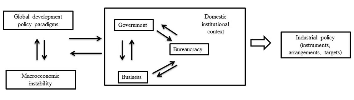 Figure 1: Flow chart summarising the book’s main argument. Source: M Kerem Coban.
Chapter Two focuses on the longue durée between 1923 and 1980. From the ashes of incessant wars that ruined the already unsophisticated infrastructure and demographic challenge, the new Republic had to build a new nation. Yet the rise of the state interventionist era in the 1930s drove policymakers towards the first industrialisation plan and the opening of many industrial sites across the country. When the Democrat Party assumed power, the interventionist, planning-based industrial policy was scrutinised for liberalisation that even included state-owned enterprises to be released to set up their own prices (73).
At the same time, business was encouraged to invest. For example, the fruits of these included Otosan or BOSSA (75). Between 1960 and 1980, the authors underline the second planning period with the establishment of the State Planning Organisation (SPO). SPO boosted bureaucratic and planning capacity and capabilities for disciplined, systematic industrial policy during the era of import-substitution.
Between 1980 and 2000 […] Turkey shifted to export-led growth and liberalised trade and financial flows. These shifts had profound implications for bureaucracy
The third chapter examines demoted industrial policy between 1980 and 2000 when Turkey shifted to export-led growth and liberalised trade and financial flows. These shifts had profound implications for bureaucracy: SPO was sidelined, parallel bureaucratic networks of Ozal were implanted with the opening of new offices or agencies. Consequently, the role of state became less coherent, as political uncertainty driven by unstable coalitions eroded the market-shaping role of the state. The financial sector did not help industrial policy, since banks were dominantly financing chronic budget deficits during a period of high inflation (111). What is more, business, including Islamic conservative SMEs in Anatolia, reduced or ignored investments in manufacturing given the clientelist state-business relations that incentivised construction, real-estate development (115), emphasis in original). Finally, the external conditions were not disciplinary: accession to the Customs Union with the European Union and the World Trade Organization ruled out export support and import restricting measures, among other trade regulatory instruments.
The fourth chapter claims that industrial policy retreated between 2001 and 2009. The first years of this period was marked by political instability and a local systemic banking crisis and its resolution, and Justice and Development Party (AKP in Turkish) assumed power. During this period, industrial policy was dominated by institutionalisation of the regulatory state and the privatisation of state-owned enterprises, the establishment of autonomous regulatory agencies and are structured banking sector. While the regulatory capacity of the state increased, privatisation and the regulation of the market were highly politicised. For example, “a major cycle of gas privatisation saw ‘politically connected persons’ winning fifteen out of nineteen metropolitan centres and serving 76 percent of the population” (161). In such a politically compromised setting, which was accompanied by the institutionalisation of the capital inflow-dependent credit-led growth model that prioritised “rent-thick” sectors, industrial policy could not flourish.
While the regulatory capacity of the state increased, privatisation and the regulation of the market were highly politicised.
The fifth chapter locates the policy within the global ideational and political economic context that marks the return of industrial policy in various forms. In line with policy documents such as the 11th Development Plan, horizontal measures, private and public R&D spending on high-tech initiatives, electric vehicle manufacturing attempt, and most notably the advancements in defence sector have constituted the revival of industrial policy. At the same time, the authors point to several challenges such as eroded academic research and quality and a lack of investment in ICT skills. Additionally, R&D subsidies or other industrial policy measures require thorough performance criteria and measurement to discipline actor behaviour and regulate the incentive structures.
Industrial Policy in Turkey is a timely contribution to the current debate. Its historical account and analysis of current policies, instruments, and the potential trajectory of industrial policy are its main strengths. Still, there are several caveats. First, the book’s framework is not systematic, which causes some confusion. For example, the book does not demonstrate a convincing link between the role and impact of autonomous agencies on industrial policy. Second, the book leaves the reader with more questions than answers, one of which relates to the effect of bureaucratic fragmentation in shaping industrial policy. Another is around the implications of state-business for bureaucracy, and consequently, industrial policy.
The book leaves the reader with more questions than answers, one of which relates to the effect of bureaucratic fragmentation in shaping industrial policy.
Third, the trajectory of industrial policy cannot be considered independently from the shifts in growth models. Yet the fact these shifts occur because the country depends on hard currency earnings for capital accumulation and to finance consumption and investments: Turkey either relies on capital flows or export earnings, in addition to tourism and (un)recorded (illicit) flows. Pendulums between these channels imply that the country cannot design and implement disciplined, systematic industrial policy. Put differently, there are macroeconomic and financial structural impediments against generating hard currency earnings. Industrial policy is one of the remedies, however, the macroeconomic and structural transformative consequences of the latest episode of emphasis on industrial policy and the export-driven growth experiment in Turkey are yet to be seen.
Finally, and perhaps most importantly, the book tends to relegate a core problem of coordination, long-term policy design and implementation to “governance issues”. Deeper cultural, social, political and economic factors determine the clientelist state-business relations and their effect on bureaucracy and bureaucratic autonomy. Such deeper ties have been masked by instrumentalised “democratisation reforms” or higher economic growth rates in the previous years. In this context, is the more critical problem the purposefully immobilised or challenged infrastructural power to coordinate societal actors? If that is true, then should we make interdisciplinary attempts to identify this problem’s core determinants?
Note: This interview gives the views of the author, and not the position of the LSE Review of Books blog, or of the London School of Economics and Political Science.
Image credit: Chongsiri Chaitongngam on Shutterstock.
Global Supply Chains and U.S. Import Price Inflation

Inflation around the world increased dramatically with the reopening of economies following COVID-19. After reaching a peak of 11 percent in the second quarter of 2021, world trade prices dropped by more than five percentage points by the middle of 2023. U.S. import prices followed a similar pattern, albeit with a lower peak and a deeper trough. In a new study, we investigate what drove these price movements by using information on the prices charged for products shipped from fifty-two exporters to fifty-two importers, comprising more than twenty-five million trade flows. We uncover several patterns in the data: (i) From 2021:Q1 to 2022:Q2, almost all of the growth in U.S. import prices can be attributed to global factors, that is, trends present in most countries; (ii) at the end of 2022, U.S. import price inflation started to be driven by U.S. demand factors; (iii) in 2023, foreign suppliers to the U.S. market caught up with demand and account for the decline in import price inflation, with a significant role played by China.
Methodology
We use bilateral trade data for all shipments of disaggregated products from an exporting country to an importing country for fifty-two countries, which make up more than 90 percent of U.S. imports. We divided the value of each HS10-country observation by the quantity to form the unit value, which is our measure of the price. We estimate the average change in log prices for each exporter and each importer for each product in each quarter, all relative to the global median price. We refer to the worldwide median as the “global common shock,” the exporter average price change less the median change as the “idiosyncratic supply shock,” and the importer average price change less the median one as the “idiosyncratic demand shock.” Our forthcoming publication in the American Economic Association (AEA) Papers and Proceedings provides more details of this methodology. Below, we summarize our findings, and for this post, we extend the sample period to include 2023.
U.S. Aggregate Import Prices
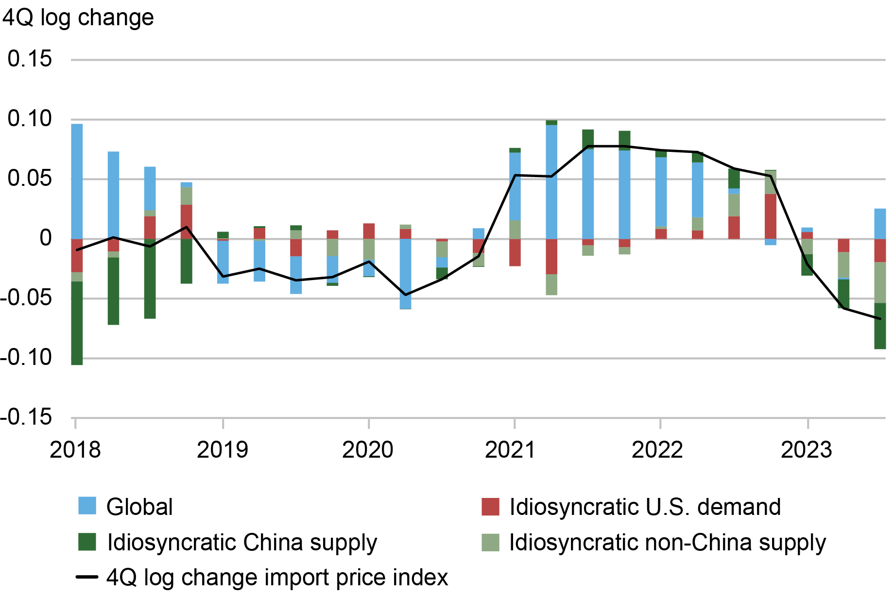
The chart below plots the decomposition of the changes in aggregate U.S. import prices and shows the sources of the rise and fall of aggregate import price inflation, corresponding to the black line. We also plot each of the three components (common, idiosyncratic U.S. demand, and idiosyncratic export supply price shocks), where we further split the export supply price shock into the element driven by China (dark green) and other exporters to the U.S. (light green). The sum of the colored bars equals the change in the aggregate import prices.
Global Factors Drive Growth in U.S. Import Prices after COVID-19 until Mid-2022
 Source: Authors’ calculations based on data from UN COMTRADE and GTAS.
Note: See Amiti, Itskhoki, Weinstein, “What Drives U.S. Import Price Inflation?” for details.
The chart shows that import price inflation was driven mainly by the global common shock (blue bars) until the second half of 2022. Import price inflation rose to 8 percent in the second half of 2021 and fell to -6 percent by the third quarter of 2023. The global common factor (blue bars) played a dominant role in the aftermath of COVID-19 when all countries struggled to re-open their economies. However, by the end of 2022, the global common factor stopped affecting import price inflation. Instead, idiosyncratic U.S. demand and later price reductions by the major exporters to the U.S. played the dominant role in price fluctuations.
In particular, idiosyncratically strong demand in the U.S. maintained high import inflation rates in the second half of 2022. However, this demand effect was short-lived and fell to close to zero at the start of 2023. These findings suggest that most import price inflation was common to all countries until the middle of 2022 and, therefore, cannot be explained by distinctive U.S. policies or policies peculiar to our trading partners. In other words, COVID-19 was a worldwide shock that affected import prices in all countries approximately equally.
As supply chain pressures have eased, import prices have fallen, and we see that idiosyncratic supply shocks have been responsible for the price declines in 2023. Perhaps in response to the high import prices that emerged after COVID-19, the U.S.’s leading suppliers ramped up production and dropped prices. The dark green bars indicate that much of the drop in import prices is due to China, whose exporters dropped prices by more than those in other countries. These patterns suggest that the U.S. import price inflation was not due to a poor choice of trading partners.
In the wake of COVID-19, import prices rose in the U.S. because they rose everywhere and not because of idiosyncratic U.S. demand or decisions made by our leading import suppliers. When U.S. import prices fell in 2023, it was mostly the product of large price drops by China and our other major import suppliers. Some of the decline in the U.S. import prices in 2023 may be due to the relative strength of the U.S. dollar, but we find little correlation between trade-weighted USD and import price inflation over the rest of the sample period.

Mary Amiti is the head of Labor and Product Market Studies in the Federal Reserve Bank of New York’s Research and Statistics Group.
Oleg Itskhoki is a professor of economics at the University of California, Los Angeles.
David E. Weinstein is the Carl S. Shoup Professor of the Japanese Economy at Columbia University.
How to cite this post:
Mary Amiti, Oleg Itskhoki, and David E. Weinstein, “Global Supply Chains and U.S. Import Price Inflation,” Federal Reserve Bank of New York Liberty Street Economics, March 4, 2024, https://libertystreeteconomics.newyorkfed.org/2024/03/global-supply-chai....

Pass‑Through of Wages and Import Prices Has Increased in the Post‑COVID Period

High Import Prices along the Global Supply Chain Feed Through to U.S. Domestic Prices
Disclaimer
The views expressed in this post are those of the author(s) and do not necessarily reflect the position of the Federal Reserve Bank of New York or the Federal Reserve System. Any errors or omissions are the responsibility of the author(s).
Ecological economics and modern monetary economics need each other
Ecological economics and modern monetary economics need each other Steven Hail Here are three things that ecological economists often do not get quite right about…
Can Electric Cars Power China’s Growth?

China’s aggressive policies to develop its battery-powered electric vehicle (BEV) industry have been successful in making the country the dominant producer of these vehicles worldwide. Going forward, BEVs will likely claim a growing share of global motor vehicle sales, helped along by subsides and mandates implemented in the United States, Europe, and elsewhere. Nevertheless, China’s success in selling BEVs may not contribute much to its GDP growth, owing both to the maturity of its motor vehicle sector and the strong tendency for countries to protect this high-profile industry.
China’s BEV Industry
The International Energy Agency’s (IEA) EV Outlook documents the policies that fostered China’s BEV industry. It notes that the government introduced incentives to purchase BEVs (subsidies to consumers, tax exemptions), implemented industrial policies (mandates to produce new energy vehicles, subsidies to producers), and undertook infrastructure investments in public charging stations. Justifications for this expensive push include advancing the country’s design and manufacturing skills, cutting oil imports, reducing urban air pollution, and addressing climate change.
Domestic production responded. Output of BEVs increased from around 1 million vehicles in 2020 to just over 6 million in 2023, with domestic BEV sales accounting for 23 percent of the passenger car market last year.
China’s BEV Production Has Increased Dramatically
Millions of units (12-month sums)
{"data":{"groups":[],"labels":false,"type":"line","order":"desc","selection":{"enabled":false,"grouped":true,"multiple":true,"draggable":true},"xFormat":"%m\/%d\/%Y","x":"Date","rows":[["Date","Units"],["9\/30\/2020","0.664"],["10\/31\/2020","0.733"],["11\/30\/2020","0.811"],["12\/31\/2020","0.917"],["1\/31\/2021","1.043"],["2\/28\/2021","1.131"],["3\/31\/2021","1.257"],["4\/30\/2021","1.372"],["5\/31\/2021","1.478"],["6\/30\/2021","1.605"],["7\/31\/2021","1.762"],["8\/31\/2021","1.933"],["9\/30\/2021","2.118"],["10\/31\/2021","2.299"],["11\/30\/2021","2.501"],["12\/31\/2021","2.732"],["1\/31\/2022","2.932"],["2\/28\/2022","3.104"],["3\/31\/2022","3.292"],["4\/30\/2022","3.356"],["5\/31\/2022","3.532"],["6\/30\/2022","3.786"],["7\/31\/2022","4.005"],["8\/31\/2022","4.259"],["9\/30\/2022","4.521"],["10\/31\/2022","4.754"],["11\/30\/2022","4.951"],["12\/31\/2022","5.101"],["1\/31\/2023","5.026"],["2\/28\/2023","5.114"],["3\/31\/2023","5.229"],["4\/30\/2023","5.447"],["5\/31\/2023","5.587"],["6\/30\/2023","5.645"],["7\/31\/2023","5.718"],["8\/31\/2023","5.755"],["9\/30\/2023","5.74"],["10\/31\/2023","5.806"],["11\/30\/2023","5.923"],["12\/31\/2023","6.116"],["1\/31\/2024","6.28"]]},"legend":{"show":false,"position":"bottom"},"axis":{"rotated":false,"x":{"show":true,"type":"timeseries","localtime":true,"tick":{"centered":false,"culling":{"max":""},"fit":true,"outer":true,"multiline":false,"multilineMax":0,"format":"%Y","values":["1\/31\/2020","1\/31\/2021","1\/31\/2022","1\/31\/2023","1\/31\/2024"]},"label":{"text":"","position":"outer-center"},"format":"%Y-%m-%d"},"y":{"show":true,"inner":false,"type":"linear","inverted":false,"tick":{"centered":false,"culling":false},"padding":{"top":3,"bottom":0},"primary":"","secondary":"","label":{"text":"","position":"outer-middle"},"min":0,"max":7},"y2":{"show":false,"inner":false,"type":"linear","inverted":false,"padding":{"top":3},"label":{"text":"","position":"outer-middle"}}},"chartLabel":"Millions of units (12-month sums)","padding":{"auto":true},"color":{"pattern":["#61AEE1","#B84645","#B1812C","#046C9D","#9FA1A8","#DCB56E"]},"interaction":{"enabled":true},"point":{"show":false},"tooltip":{"show":true,"grouped":true},"grid":{"x":{"show":false,"lines":[],"type":"indexed","stroke":""},"y":{"show":true,"lines":[],"type":"linear","stroke":""}},"regions":[],"zoom":false,"subchart":false,"download":true,"downloadText":"Download chart","downloadName":"chart","trend":{"show":false,"label":"Trend"}}
Source: China Passenger Car Association/Haver.
The IEA’s 2023 report recounted how hundreds of Chinese firms entered the field when the subsidies and incentives were implemented, but that most went bankrupt, leaving some dozen firms to produce BEVs in a broad price range. They describe a market with some vehicles sold at very low prices, with the average price of the smallest BEVs in China at around $10,000 in 2022, compared to $35,000 in Europe and the United States, albeit with a substantially shorter battery range. The price differential is also evident in the SUV segment, with the average price in China at $35,000, much lower than the $65,000 average in the other two markets even though the average ranges are similar across the three regions.
Recipe for Growth?
While technologically advanced, the extent that BEVs can contribute to GDP growth is limited by the maturity of the motor vehicle industry, with passenger car sales having peaked in 2017. This is a restraining factor as BEVs do not represent an innovation that creates new demand, like the introduction of personal computers or cell phones. Instead, they’re a new version of a familiar product whose sales may not grow much beyond current levels.
BEVs might still increase the industry’s contribution to GDP growth if customers switched away from imports to domestically produced vehicles. The potential gains, though, are likely to be small, as China used very high tariffs to force foreign firms to open local plants, with the requirement that they have a domestic partner. The arrangement means that foreign firms keep a share of the profits from their Chinese operations while the value-add embedded in domestic motor vehicle sales is almost entirely created in China.
Not having a meaningful number of imports implies that any switch away from passenger cars running on internal combustion engines (ICE) to BEVs will have winners and losers inside China, reminiscent of a zero-sum game, but will not do much to lift GDP. If anything, technological improvements in batteries that lower the average price of motor vehicles, while a benefit to consumers, will shrink the output of the motor vehicle sector unless matched by a corresponding increase in unit sales.
One bright development for China’s economy has been an increase in BEV exports. Foreign sales of these vehicles have risen from around 250,000 units in 2020 to 500,000 units in 2021, 1.0 million units in 2022, and 1.5 million units in 2023, according to data from China’s General Administration of Customs. Unfortunately, the UN Comtrade database, with its breakdown of exports by country (the HS code for BEVs is 870380) available through 2022, seen in the chart below, shows the need to adjust these numbers. It is apparent that the category includes both BEVs and cheap electric carts, with the value of vehicles shipped to Bangladesh, India, the Philippines, and Thailand averaging just $2,500 in 2022—compared to $30,000 for vehicles going to Europe. It makes sense, then, to subtract out sales to these four countries to get a better measure of BEV exports and, indeed, the average value without these four is close to Europe’s average value. Such an adjustment raises the 2022 growth rate for BEV exports (122 percent versus 90 percent) but lowers the volume of exports to around 700,000 units. The 2023 breakdown is not available, but the adjusted total will likely be over 1 million units.
China’s BEV Exports to Europe Have Surged
Thousands of units
{"data":{"groups":[],"labels":false,"type":"line","order":"desc","selection":{"enabled":false,"grouped":true,"multiple":true,"draggable":true},"rows":[["Europe","Emerging economies","Australia and New Zealand","Middle East","Other"],["48","127","1","1","17"],["226","190","15","14","55"],["436","255","49","81","123"]]},"axis":{"rotated":false,"x":{"show":true,"type":"category","localtime":true,"tick":{"centered":false,"culling":false,"fit":true,"outer":true,"multiline":false,"multilineMax":0},"label":{"text":"","position":"outer-center"},"categories":["2020","2021","2022"]},"y":{"show":true,"inner":false,"type":"linear","inverted":false,"tick":{"centered":false,"culling":false},"padding":{"top":3,"bottom":0},"primary":"","secondary":"","label":{"text":"","position":"outer-middle"},"min":0,"max":500},"y2":{"show":false,"inner":false,"type":"linear","inverted":false,"padding":{"top":3},"label":{"text":"","position":"outer-middle"}}},"chartLabel":"Thousands of units","padding":{"auto":true},"color":{"pattern":["#61AEE1","#B84645","#B1812C","#046C9D","#9FA1A8","#DCB56E"]},"interaction":{"enabled":true},"point":{"show":false},"legend":{"show":true,"position":"bottom"},"tooltip":{"show":true,"grouped":true},"grid":{"x":{"show":false,"lines":[],"type":"indexed","stroke":""},"y":{"show":true,"lines":[],"type":"linear","stroke":""}},"regions":[],"zoom":false,"subchart":false,"download":true,"downloadText":"Download chart","downloadName":"chart","trend":{"show":false,"label":"Trend"}}
Source: UN Comtrade.
Notes: Emerging economies include Bangladesh, India, the Philippines, and Thailand. Middle East includes Israel, Jordan, and the UAE.
Protectionism
The extent of export gains for China depends on both the share of BEVs purchased abroad and China’s share of these BEV sales. Consider Europe, which received over half of China’s BEV exports in 2022, 436,000 units. (Note that exports to the United States were trivial due to very high U.S. tariffs.) The European Automobile Manufacturers Association estimates that BEV sales in Europe equaled 1.2 million in 2021 and 1.6 million in 2022, with total sales of motor vehicles dipping from 11.8 million to 11.3 million. Given the rising popularity of BEVs (increasing from 10 percent to 14 percent of the market) and China’s higher share of that region’s BEV sales (17 percent to 28 percent), a quick calculation shows that China’s BEV share of total vehicle sales doubled from 2 percent to 4 percent in one year. Assuming that China’s exports to Europe grew at the same rate as its total BEV exports, then Chinese vehicles made up 35 percent of Europe’s higher BEV sales in 2023, accounting for 5.5 percent of total motor vehicle sales in the region.
Such gains may soon flatten out, both from greater competition as European plants work to catch up and from political pressure to put a cap on China’s exports. China itself is a case study of a government protecting a favored domestic industry, with the U.S.-Japan Voluntary Export Restraint (VER) program in the early 1980s being another. The oil shocks of 1973 and 1979 created a competitive advantage for Japanese firms that had specialized in fuel-efficient vehicles. The VER program was designed to protect a highly visible U.S. manufacturing industry under an agreement that Japanese firms would have to open plants in the United States in order to sell more to the U.S. market. These experiences suggest that Chinese firms, whether producers of BEVs or the batteries they run on, will face implicit and explicit pressure to build facilities in foreign markets if they want to grow their sales.
Significant Gains Elsewhere
While BEVs may have limited potential to increase the motor vehicle sector’s contribution to Chinese GDP, that does not diminish the other significant gains from the policies that fostered the industry, such as the profits to be made from any new foreign operations, the technological and manufacturing spillovers to the rest of the economy, and the replacement of imported petroleum products with domestic renewable energy. Indeed, the EIA’s 2023 EV report forecasts that China’s adoption of electric vehicles will lower its crude oil consumption in 2030 by 2 million barrels per day, which is equal to 12 percent of the country’s current liquid fuel consumption.

Thomas Klitgaard is an economic research advisor in International Studies in the Federal Reserve Bank of New York’s Research and Statistics Group.
How to cite this post:
Thomas Klitgaard, “Can Electric Cars Power China’s Growth?,” Federal Reserve Bank of New York Liberty Street Economics, February 28, 2024, https://libertystreeteconomics.newyorkfed.org/2024/02/can-electric-cars-....

Can China Catch Up with Greece?


Is China Running Out of Policy Space to Navigate Future Economic Challenges?
Disclaimer
The views expressed in this post are those of the author(s) and do not necessarily reflect the position of the Federal Reserve Bank of New York or the Federal Reserve System. Any errors or omissions are the responsibility of the author(s).
Forecasting UK inflation in the presence of large global shocks
Dario Bonciani and Johannes Fischer

The UK economy has been hit by significant terms-of-trade shocks, most notably the rise in energy prices following the Russian invasion of Ukraine. These shocks have created substantial and persistent inflationary pressure in many countries. Such upheavals bring increased uncertainty about the future, making macroeconomic forecasting more challenging. In this post, we assess the forecasting performance of a state of the art empirical model, of the type commonly employed in academic research and policy institutions. This model is not used to produce the Monetary Policy Committee’s (MPC’s) forecast but has been used periodically within the Bank of England including as a cross-check to the main forecast. Specifically, we assess its performance in predicting UK inflation out of-sample at key dates around the start of the war in Ukraine. The model performs well in forecasting short-term inflation, but it struggles to fully capture inflation persistence over the longer term.
Methodology
To conduct our forecasting analysis, we have employed a Bayesian Vector Autoregressive (BVAR) model. These types of models have gained widespread popularity in academia and central banks for their flexibility and strong forecasting abilities, as evidenced by studies like Bańbura et al (2010) and Angelini et al (2019).
In essence, this empirical framework encompasses a series of linear equations designed to model the interdependencies and dynamics of macroeconomic variables. Further details on BVARs can be found here. Our specification includes 20 variables. Among these, 15 are specific to the UK economy, including the consumer prices index (CPI), real gross domestic product (GDP), the Bank Rate, and specific components of CPI, such as energy and food. Additionally, we incorporate global variables in the model, including world real GDP, global trade, and world CPI. Our model specification was used in a recent speech by Catherine L Mann, an external member of the Bank of England’s MPC. In her speech, she highlights how including periods of high inflation, such as 2022 Q1–2023 Q2, in the estimation sample affects the inflation forecasts of the BVAR.
The BVAR model relies on historical regularities between the included variables to produce forecasts. To capture these historical regularities, we estimate the model parameters using quarterly data from 1992 to 2019. To produce our BVAR forecasts, we make the additional assumption that the energy and food CPI components in the model are expected to follow exactly the same path as implied by real-time market futures curves (which will be influenced by financial market participants’ expectations about future prices). This assumption enables our model to factor in information about the latest events affecting food and energy prices. This assumption is necessary as we want the model to have all the information available at each point in time. Using the estimated historical regularities along with real-time information on the futures curves for energy and food prices, we then generate out-of-sample inflation forecasts at various points in time. In this post, we focus on the forecasts implied by the model before and after the onset of the Ukrainian conflict.
Empirical model estimated on pre-pandemic data
Chart 1 presents three panels illustrating inflation forecasts based on real-time data at two distinct time points: 31 January 2022 and 30 April 2022. The purple lines represent the BVAR forecasts, while the dashed lines depict the evolution of actual inflation. For comparison, we also include the median inflation forecast from the Market Participants Survey results as green dots. Finally, the shaded areas denote the statistical uncertainty surrounding the BVAR forecasts.
Chart 1: Comparing inflation forecasts at different points in time

In January 2022, as the threat of the Russian invasion became more likely, the BVAR forecast (upper Chart 1 panel) projected inflation to peak at 8% in November 2022. In comparison, professional forecasters expected inflation to peak at 6%, 2 percentage points lower than the BVAR.
Two months after the beginning of the Russian invasion, in April 2022 (lower Chart 1 panel), both the BVAR and professional forecasters had adjusted their forecasts upwards to reflect the increase in energy prices. In the short term (the first two quarters), the BVAR model closely tracked realised inflation. However, inflation proved more persistent than the model’s historical regularities and futures curves about food and energy prices could predict. The gap between the forecast of the BVAR and that of professional forecasters that existed in January disappeared almost completely by the end of April. One potential explanation for the initial difference in forecasts (and its disappearance) could be that professional forecasters had not considered the Russian invasion of Ukraine to be as likely as financial market participants had. Finally, professional forecasters also did not anticipate inflation remaining high for an extended period.
Overall, the BVAR model’s forecasts implied high rates of inflation before the Russian invasion of Ukraine but missed realised inflation by several percentage points. Once the Russian invasion had begun, the inflation peak of the BVAR forecast is close to the eventual peak.
Including post-pandemic information
Lastly, we examined whether the persistent rates of inflation seen over the past two years may significantly affect future BVAR forecasts, as argued in the above-mentioned speech by Catherine L Mann. To do so, we re-estimated the model with data that includes the run-up in inflation up until 30 April 2023, excluding the outlier data during the pandemic years (2020–21), as per the methodology in Cascaldi-Garcia (2022). The out-of-sample forecast with the data available at this point in time slightly increased the inflation persistence. Interestingly, over the full forecast horizon, the predictions from the BVAR model and professional forecasters aligned very closely.
Chart 2: Does post-pandemic data affect the inflation forecast?

Conclusion
Returning to our initial question, to what extent a linear model can predict inflation in the face of large terms-of-trade shocks. Prior to the war in Ukraine the model forecasted inflation significantly below its eventual realisation. This is not surprising because the model could not have foreseen the extent of the energy price increase associated with the war. Following the start of the war, when the energy price increase was realised, the BVAR model performed well in forecasting inflation in the nearer term despite its relative parsimony. However, it struggled to fully capture the inflation’s persistence over the longer term. Using data realisations from 2020 onwards to estimate the BVAR parameters can potentially help better capture the persistence of inflation in the future. Our analysis suggests that a linear model such as the BVAR can still prove to be robust for forecasting even in a turbulent macroeconomic environment.
Dario Bonciani and Johannes Fischer both work in the Bank’s Monetary Policy Outlook Division.
If you want to get in touch, please email us at bankunderground@bankofengland.co.uk or leave a comment below.
Comments will only appear once approved by a moderator, and are only published where a full name is supplied. Bank Underground is a blog for Bank of England staff to share views that challenge – or support – prevailing policy orthodoxies. The views expressed here are those of the authors, and are not necessarily those of the Bank of England, or its policy committees.
Inflation and Power
It was a mistake to accept a ‘reference price’-determination process for basic commodities led by finance
const trinityScript = document.createElement('script'); trinityScript.setAttribute('fetchpriority', 'high'); trinityScript.src = 'https://trinitymedia.ai/player/trinity/2900011009/?pageURL=' + encodeURIComponent(window.location.href); document.currentScript.parentNode.insertBefore(trinityScript, document.currentScript);
There are strong interrelations between economic policy, culture, and power relations in society. This is quite evident in the restrictive monetary policies undertaken by central banks the world over when confronted with the recent inflationary outbursts.
Restrictive monetary policies are a standard answer to inflation. But they are not costless, exerting a downward pressure on output and employment. Thus, two questions arise: are they the correct answer in general? And are they, in this specific situation?
My answer is different from the mainstream one. The theoretical background pointing to restrictive monetary policies as the general answer to inflation does not have general validity, though it may hold in some specific circumstances. And, when confronted with the present inflationary episode, there are other policies we should consider first.
An old-fashioned quantitative theory of money is still often referred to (or implicitly relied on) by the media, and occasionally by professional economists, in support of the argument that price increases are caused by increases in the amount of money in circulation. But, as Kaldor once pointed out to Friedman, the causal link may go in the opposite direction: when prices increase, banks may be led to increase the money amount of their loans, thus increasing the supply of bank money. Moreover, when confronted with increasing aggregate demand, aggregate output too may increase, unless we are in a situation of full utilization of productive capacity, which is very rare – and certainly not our present condition.
But for sure there is an avenue through which restrictive monetary or fiscal policies exert downward pressure on inflation, and it is through the impact of a reduction in employment on the bargaining power of workers, hence on wage dynamics. Thus, these policies are an instrument of redistributive policies, not a class-neutral policy choice. (In this respect we can also notice that they favor the profits of banks, insurance companies, and financial institutions in general).
In sum, restrictive monetary policies should be considered with caution when confronted with output inflation. They are instead, quite often, a useful tool for countering asset inflation.
In the present situation, we are confronted with a multi-faceted inflationary outburst. The Covid pandemic first, then the war in Ukraine, ignited inflation by disrupting global supply chains, then gas and agricultural markets. Now the difficulties of navigation through the Gulf of Aden and the Red Sea increase transport costs and further disrupt supply chains.
Simplifying a complex matter, we can say that the restructuring of supply chains is certainly not favored by restrictive monetary policies. And, as far as gas and agricultural markets are concerned, there has been a clear overreaction of prices to the underlying admittedly difficult situation (with oil markets also displaying excess variability). Such an overreaction – the main element in the inflationary outburst – is mainly due to the financial markets that play a basic role in the price-determination process for these commodities. Financial markets do not behave in accordance with the efficient financial markets theory, driving prices in such a way as to reflect the underlying real situation: they are bent to overreact, driven by speculation.
It was a mistake – an enormous mistake – to accept a ‘reference price’-determination process for basic commodities led by finance, while direct (and often long-term) bargaining between companies at much lower prices inflates the companies’ profits, with selling prices for final products linked (by informal collusion if not by formal rules, as is the case for electricity) to the reference price. Countering this situation requires active anti-trust policies, a revision of some regulations, and more generally an active policy aiming at a retrenchment of finance (and the financialization of commodities in particular), whose growth as a percentage of GDP over the past few decades is the main cause of the growing instability of the world economy.
Such policies imply a wide redistribution of power in the economy and in society at large. They have no possibility of being implemented if not supported by a widespread recognition of the failures of neoliberal theories and policies, and this in turn requires turning upside down some established pillars of mainstream economic culture. We should recognize that culture and politics, in their more general meaning, have a deep influence on the formation of economic policy strategies.
Alessandro Roncaglia is Emeritus Professor of Economics at Sapienza University in Rome and a member of the Accademia Nazionale dei Lincei. He is the author of many books and articles. His Power and Inequality: A Reformist Perspective is just appearing in the INET “Studies in New Economic Thinking” book series with Cambridge University Press.
Nominal Versus Real Models
Modern economics uses “scientific” methodology, under the assumption that economic laws are invariant across time, space, and society. In previous posts, we saw how this leads to loss of precious insights about money gained from historical experiences (Monetary Economies: A Historical Perspective, Lessons from Monetary History: The Quality-Quantity Pendulum). In this post, we will discuss the modeling strategy we will use to derive lessons from history which extend beyond the particular historical context from which they are derived. Modern Economics uses nominal models (the as-if methodology of Friedman) which make it impossible to understand the role of money within an economy. We plan to use the alternative – realism – combined with Agent Based Models, to capture essential features of monetary economies.
Models are simplified representations of reality. When considering monetary history, the factors driving changes are notably intricate. Over the 20th century, the monetary system underwent significant transformations. World War I marked the breakdown of the gold standard, followed by unsuccessful attempts at restoration. World War II further hindered restoration efforts, leading to the Bretton Woods agreement and the adoption of a gold-backed dollar standard. Nixon’s actions in 1971 severed the link between the dollar and gold, ushering in an era of floating currencies detached from commodities. Distilling broader lessons from the complexity of historical specifics necessitates a methodological approach centered on models. Models abstract from specific historical details to illuminate structures which may be widely applicable across various historical and temporal contexts.
In this text, we will be using realist models – these differ greatly from the nominalist models used in conventional textbooks of economics. The difference can be explained as follows. Our world comprises observable phenomena as well as underlying structures that produce these observations. Nominalism holds that models should focus solely on explaining observables, disregarding whether they accurately reflect hidden reality. This notion, though counterintuitive, emerged due to the belief that hidden reality is unknowable, making the pursuit of matching it futile. Instead, nominalism advocates for assessing a model’s success based on its ability to explain observed phenomena. Conversely, realist models strive to mirror the hidden reality behind observations.
Friedman’s essay on “The Methodology of Positive Economics” strongly advocates the use of nominal models. This methodological principle has been widely accepted by economists. Friedman illustrates nominal models with the example of a skilled pool player. He suggests that even if the player lacks any understanding of physics, assuming knowledge of the laws of physics can lead to accurate predictions of their shots. In essence, the player behaves as if they comprehend physics, making successful shots based on calculations, despite their ignorance of the underlying principles of physics. This is known as the “as-if” methodology, and it is the dominant approach to models in modern economics.
In contrast, realist approaches reject such assumptions. For the pool player, a realist model might study his past experiences, and his skills at different types of shots. Realism aims to understand the internal workings of hidden reality, while nominalism accepts models that predict outcomes, without concern about matching hidden reality. Friedman developed his as-if theory in response to empirical surveys which showed the most firms do not maximize profits. He argued that the assumption of profit maximization, even if it did not match the motivations of the managers of the firms, should be assessed on the basis of its ability to predict decisions about hiring and production. However, by now, this methodology has been in use for several decades, and it has led to repeated failures. A good fit to observations for a particular finite set of data is not a guarantee of the validity of a model. It can, and often does, happen by chance. For a more detailed discussion of the superiority of real models to nominal models in the context of econometrics, see “A Realist Approach to Econometrics” (bit.ly/azrae)
We will use a recently introduced modeling strategy — Agent-Based Models (ABMs) – which has not made its way into mainstream methodology. ABM models have multiple agents – laborer, producer, shopkeeper, government, etc. – each of which has their own economic decisions to make, and behavioral patterns. This strategy has become feasible because of the vastly increased computational power now available, which permits us to run simulations and compute outcomes. The foundations of modern economic methodology, established around the mid-20th century, relied on simplifying assumptions to facilitate manual computations. For example. Leading macroeconomic models have only one agent, who has perfect foresight. Why? Because computations by hand would be impossible with two or more agents. At a Congressional inquiry into the failure of economists to predict the Global Financial Crisis of 2007, Solow testified that the GFC was caused by large scale deception and fraud. Macroeconomists could not predict it because these are impossible in models with only one agent. In contrast, models with heterogenous behavior are much better at capturing the complex internal structures of modern economies, in accordance with the principle of realist models.
Using ABMs, we can capture three Keynesian insights, all of which are essential for the understanding of money, and all of which are missing from conventional textbooks:
Complexity: This technical term refers to a situation where the group behaves very differently from the individuals within the group. For example, that even though laborers and the firms which hire them may seek to lower the real wage, they can only negotiate on the nominal wage. The real wage involves the price level of the economy which is out of their control. Keynes argued that lowering nominal wages at the micro level throughout the group may end up increasing the real wage – a perfect example of complexity. This phenomenon is beyond the reach of conventional economic theory because the textbook models are oversimplified to prevent the occurrence of complexity.
Radical Uncertainty: In a model with heterogeneity, each agent has access to a limited amount of information. The economic outcomes depend on the actions of all agents, which can never be known to the agents. As a result, the agent operates in an environment where the outcomes of the decisions he takes are not predictable. Standard textbook models use intertemporal optimization, where the agent knows his future incomes, potential consumption bundles and prices. This is simply impossible in our agent-based models. Similarly, profit maximization is impossible for firms because they incur production costs in current period, but will produce and sell goods in the next period. The price at which they can sell will depend on decisions others make, and cannot be predicted. So profits are subject to radical uncertainty, and cannot be maximized.
Non-Neutrality of Money: Once we take into account heterogeneity and uncertainty, new insights into the role of money emerge, not available in conventional textbooks. Workers save money, and firms acquire money profits, but, due to radical uncertainty, no one knows what the value of money will be in the next period. A stable value of money allows for some degree of planning, but the QQ-pendulum shows that this stability cannot be relied upon. The assumptions of full information made in conventional textbooks make money merely an accounting unit, which does not play an essential role in the economy. However, with radical uncertainty, and differential information and behavior of different agents, money plays an essential role in the economy. Workers save money as insurance against adverse outcomes in the job market, and firms save money to guard against future losses. These different motivations for holding money, and the psychological aspects which relate to public trust in the future value of money, will come to the fore in our ABM models.
To wrap up, we have discussed two types of models – nominal and real. Nominal models dominate mainstream economics, and are judged for their ability to match observations. In contrast, Realist models are judged on whether or not they match the hidden structures of reality which produce the observations. In the next section, we will build some simple realist monetary models, and show that these produce results and yield insights outside the range of orthodox monetary models.
Basics of Monetary Economies
I am planning to write a textbook on monetary economies. I will draft it section by section and chapter by chapter, and put down the drafts here for feedback and comments. The first section is given below – it is an introduction to the topic, and provides some motivation for the study, as well as hints of the methodology to be adopted.
Introduction & Motivation
A Monetary Economy is one in which the use of money is essential to the functioning of the economy. That is, without money, people would starve, and massive amounts of economic misery would result. Since monetary economies have dominated the world for centuries, this seems to us like a natural state of affairs. However, a study of history reveals that monetary economies came into existence only a few centuries ago, and eventually came to dominate the globe. Most pre-modern societies were not monetary economies. For instance, a feudal economy was not a monetary economy. The landlord owned the land, and workers on the land would receive all necessary support – food, clothing, housing, etc – from him. In return, they would work the land and produce crops, and provide other services. No money was needed for the basic necessities of life. The landlord could sell excess crops for money, and buy fineries from foreigners, but this was not essential for existence. Even today, in many areas of the world, rural subsistence economies far from urban centers are often self-sufficient, and can function without money. These non-monetary economies are excluded from the scope of our study.
Our goal in this textbook will be to clarify how monetary economies function, and how they have evolved over time. This is important because conventional modern textbooks of economics do not correctly describe monetary economies. In these textbooks, money does not serve an essential function. This point is recognized and articulated in these textbooks using the terminology “neutrality of money”. For instance, a popular textbook by Mankiw states that:
Over the course of a decade, for instance, monetary changes have important effects on nominal variables (such as the price level) but only negligible effects on real variables (such as real GDP). When studying long-run changes in the economy, the neutrality of money offers a good description of how the world works.
Exactly contrary to this, Keynes stated clearly in his landmark book entitled The General Theory of Employment, Interest, and Prices, that money plays an important role in both short and long run – it is not neutral. If money is neutral, then money plays no essential role in the economy, and so there is no essential difference between monetary and non-monetary economies. In this textbook, we will explain how money, far from being neutral, is a central driver of economic activity. Conventional textbook analysis, which takes money as neutral, leads to deep misunderstandings about modern real world economies.
The false assumption of neutrality of money led to the failure of economists to understand the causes of the Global Financial Crisis in 2007, and also to their failure to take corrective actions which could have prevented the Great Recession which followed. The battle of ideas, embodied in economic theories about money, is described in “Completing the Circle: From the Great Depression of 1929 to the Global Financial Crisis of 2007”. It is useful to briefly outline how economic theories changed over the course of the 20th Century:
- Classical Economists argued for the neutrality of money, along with other ideas, which lead to the conclusion that unemployment can only be a short-run phenomena. In the long run, unemployment will be eliminated by the workings of the free market.
- Following the Great Depression of 1929, large amounts of unemployment which persisted for long periods of time was observed. This was directly in conflict with theories of classical economics.
- Keynes then came up with a new theory, which had many revolutionary ideas, dramatically different from the assumptions of classical economics. One of the central ideas was that money is not neutral. In particular, in the labor market, the supply and demand for labor, and hence the rate of employment is strongly affected by the quantity of money available.
- Keynesian ideas came to dominate macroeconomics for about three decades following World War 2. In particular, the idea that free markets will not automatically eliminate unemployment, leads to the necessity of the government policies required to create full employment. Application of Keynesian policies led to full employment in USA and Europe for about three decades.
- The oil shock of the 1970’s led to the failure of Keynesian policies. Development of monetarism by the Chicago school of economists led to the re-instatement of pre-Keynesian ideas about the neutrality of money and the idea that free markets lead to elimination of unemployment. This came to be known as neoclassical economics, because it rejected Keynesian ideas, and went back to classical economics.
- A concerted campaign was carried out by monetarists to discredit Keynesian theories and rebuild Economics on neoclassical foundations. See Understanding Macro III: The Rule of Corporations. This was highly successful. The Monetarists went from a minority and eccentric school to the mainstream orthodoxy by the early 1990s. It became impossible to publish Keynesian and post-Keynesian views in mainstream top-ranked journals.
- Over the decade of the 1990s economic performance in the Western world became flat – fairly low growth, but no ups and downs of business cycles which had been characteristic of capitalist economies for a long time. This led to celebrations of “the Great Moderation” by the monetarists. Robert Lucas, Nobel Laureate and leading Chicago schools economist, announced triumphantly in his Presidential Address to the American Economic Association in 2003, that we economists have conquered the business cycle, and from now on, recessions will not happen.
- The Global Financial Crisis of 2007 took the economics profession by surprise, just as the Great Depression of 1929 had come as a surprise. Paul Krugman wrote the book “The Return to Depression Economics” arguing that insights of Keynes continued to be valid, and to provide deeper insights into the GFC than was available from leading neoclassical macroeconomic theories of the time. Paul Romer wrote a scathing article entitled “The Trouble with Macro” in which he argued that modern macroeconomics is based on fundamentally flawed doctrines, and leads to wildly incorrect predictions.
This is more or less the current state of affairs, as good alternatives to conventional macroeconomics are unavailable in the mainstream. The mainstream macroeconomic theories are based on assumptions which have no relation to reality. For more details, see “Why Do Economists Persist in Using False Theories?”
We will conclude this introduction to monetary economies by discussing some of the key elements of the approach we will be using. First, while mainstream macroeconomics rejected Keynesian ideas, a group of theorists known as Post-Keynesians have continued to develop the ideas of Keynes, building on his fundamental insights. This has led a branch of macroeconomics which provides much deeper insights into modern economies then the monetarism which dominates universities today. Our text borrows from these ideas. However, the critical innovation of this textbook is to study economic theory within its historical context.
As described earlier, historical events, and economic crises, have played a major role in shaping economic theories. In fact, we cannot understand economic theory as an abstraction, removed from its context. This is in conflict with the claim implicit in the use of the word “science” – lessons from study of European societies are universally applicable to all societies across time and space (see: The Puzzle of Western Social Science). In fact, all social theory is developed as an attempt to understand historical experiences of a particular society, and cannot be understood as an abstraction, detached from this historical context. Studying economics within its historical context requires a methodology radically different from that currently in use, in both orthodox and heterodox textbooks of economics currently in use around the world. We will discuss this methodology in the next section.
Monetary Policy, Illiquidity, and the Inflation Debates
The key issue is the regulation of the liquidity of all financial markets, and not just that of the banking system
const trinityScript = document.createElement('script'); trinityScript.setAttribute('fetchpriority', 'high'); trinityScript.src = 'https://trinitymedia.ai/player/trinity/2900011009/?pageURL=' + encodeURIComponent(window.location.href); document.currentScript.parentNode.insertBefore(trinityScript, document.currentScript);
The end of Quantitative Easing, and the rise in inflation since 2022 has focused attention once more on the effectiveness of monetary policy in controlling inflation. This question is framed in a way that brooks no contrary evidence: If inflation continues above target, or rises, then this is taken to mean that monetary policy is still too loose, and interest rates may need to be raised further; if inflation falls below the target level then monetary ‘tightening’ has been excessive, and may need to be loosened by a reduction in policy rates of interest.
This common view of the dilemma facing monetary policy-makers overlooks one important aspect of monetary policy, namely the effect of this policy on the liquidity of the financial system. This aspect matters for two important reasons. First of all the liquidity of the financial system determines the profile of long-term interest rates, and those rates are a crucial aspect of the monetary transmission mechanism that is supposed to make monetary policy effective in controlling inflation.
Secondly, we know that if liquidity in the financial system is reduced below a certain level, then even routine sales of long-term securities may cause a financial crisis. It was this illiquidity that lay behind the dot-com crash of 2001-2002, and subsequently the collateralised debt obligations crash of 2007-2008. By flooding the financial system with liquidity, Quantitative Easing stabilised the markets. But that is now coming to an end.
My new INET working paper explains how liquidity in the financial system rises and falls with different financing arrangements, and the mechanisms by which monetary policy influences that liquidity. It is not just all about liquidity!