macroeconomics
Measuring Price Inflation and Growth in Economic Well‑Being with Income‑Dependent Preferences

How can we accurately measure changes in living standards over time in the presence of price inflation? In this post, I discuss a novel and simple methodology that uses the cross-sectional relationship between income and household-level inflation to construct accurate measures of changes in living standards that account for the dependence of consumption preferences on income. Applying this method to data from the U.S. suggests potentially substantial mismeasurements in our available proxies of average growth in consumer welfare in the U.S.
These insights and results are based on my recent research paper coauthored with Xavier Jaravel of the London School of Economics, which is forthcoming at the Quarterly Journal of Economics.
Background
Economic theory shows that we can approximate changes in living standards using straightforward formulas known as price and quantity indices. These indices combine observed data on changes in the quantities of what we consume and the prices of those items, and are widely used by statistical offices around the world to construct measures of overall inflation in the cost of living and growth in living standards. However, this approach hinges on a crucial assumption—that the composition of what we want to buy does not shift when our incomes do (see, for example, Diewert 1993). Unfortunately, this simplifying assumption, known as homotheticity or income invariance, does not match up with a host of real-world evidence on the dependence of consumption patterns on consumer income, going as far back as the work of Engel (1857). Recent evidence on inflation inequality—the strong relationship between income and household-level measures of inflation—underscores the importance of this problem.
Insight and Method
A conceptually coherent way to measure living standards is to fix a set of prices and calculate the monetary expenditure needed, under these prices, to achieve any level of consumer welfare as it changes over time. Let us refer to this concept as real consumption, to distinguish it from the nominal expenditure of the consumer under changing prices. For instance, consider a case where all prices rise at the same 2 percent rate from one year to the next due to general inflation. Here, a consumer whose nominal expenditure has risen by 5 percent only experiences a 3 percent increase in real consumption, if we fix the prices in the initial or the final year. The key question is how to calculate the corresponding measures of inflation and real consumption growth in real-world settings in which changes in prices vary across different goods and services.
If consumer preferences are income-invariant, everyone consumes the same basket of goods and services regardless of their income level. Over time, households adjust whether to consume more or less of each good or service based on how its price changes relative to others, but these adjustments are the same for everyone. Conventional price indices tell us how to average these price changes using the expenditure shares of different goods and services, and theory tells us we need to deflate the growth in nominal expenditure based on the value of this average, which is the standard measure of inflation.
In reality, households choose different baskets of goods and services that systematically depend, among other things, on their income. Therefore, we find different inflation measures for different households when we compute the price indices using each household’s own expenditure shares, something that should not happen under the conventional assumption of income invariance. In the data, we often find lower inflation measures for richer households, meaning that prices rise more slowly for luxuries—i.e., items that are more heavily purchased by richer consumers (see, for example, Hobijn and Lagakos 2005, McGranahan and Paulson 2006, Jaravel 2019, Avtar et al. 2022, and Chakrabarti et al. 2023). Therefore, these items are becoming relatively cheaper than the others over time. This implies that, if we fix the initial prices as our basis for measuring real consumption, households that experience rising income will be shifting their consumption toward items that are accumulating relative price declines. In other words, sustained inflation bias toward necessities—goods and services favored by poorer households—means that we need relatively lower rates of growth in nominal terms to maintain the same rate of growth in real consumption. Thus, when income is growing, consumers are actually better off than that suggested by all available measures of real consumption. The conventional measures of inflation and real consumption miss this mechanism altogether. This is even true of the more recent work on inflation inequality, partially cited above, that relies on household-specific price index formulas but does not explicitly account for income dependence.
As it turns out, there is a relatively easy fix for this problem. We can correct for the effects of this income dependence in preferences simply by estimating the relationship between household income and household-specific price indices. The slope of this relationship leads to a correction factor that we need to apply to the nominal expenditure growth after it is deflated by the household’s own price index. This method is fairly easy to implement and only requires access to widely available surveys of consumption expenditure at the household level. Moreover, it can be generalized to extend to other household characteristics, such as age, family size, and education, that (1) matter for the composition of their consumption expenditure, and (2) potentially vary over time at the household level.
Application to the U.S. Data
In the paper, we apply our approach to data from the United States and quantify the magnitude of the bias in conventional measures of real consumption growth that ignore the effects of income dependence in household preferences. We build a new linked dataset providing price changes and expenditure shares at a granular level from 1955 to 2019, across the different percentiles of household (pretax) income. This dataset combines several data sources, primarily drawing from disaggregated data series available from the Consumer Price Index (CPI) and the Consumer Expenditure Survey (CEX). This new linked dataset allows us to provide evidence on the inequality in inflation over a long time horizon, thus extending prior estimates that have focused on shorter time series.
Computing inflation using income-percentile-specific price index formulas, we find that inflation inequality is a long-run phenomenon. For instance, as the chart below shows, we find that cumulative inflation from 1955 to 2019 varies substantially for households with different levels of income: while prices have inflated by a factor of around 10 for the bottom income groups, they have inflated by a factor closer to 8 at the top of the income distribution. The gap in inflation experienced by different income percentiles is sizable when compared to the overall size of inflation over the period. As such, when we look into the past from the perspective of today’s prices, we observe that (1) households were on average poorer sixty-five years ago—that is, they had stronger preferences for necessities; and (2) necessities were cheaper relative to luxuries. These empirical patterns imply that consumer welfare was higher sixty-five years ago when accounting for the dependence of preferences on income.
Inflation Inequality over the Long Run
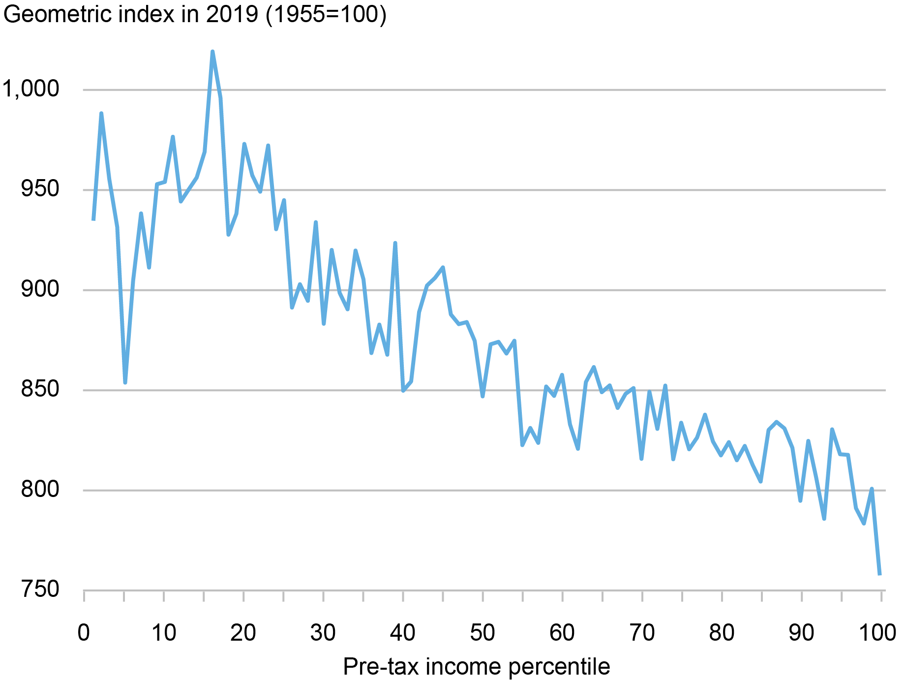
Source: Author’s calculations based on the historical linked CEX-CPI data.
Notes: This chart shows the patterns of inflation inequality in the data. It shows the cumulative inflation rates between 1955 and 2019 by pretax income percentiles.
When we apply our new method to this data, we find that the magnitude of the correction in measured welfare growth due to the effect of income-dependent preferences can be large. For example, as the chart below shows, by fixing prices in 2019 as the basis of defining real consumption, we find that the uncorrected measure underestimates average real consumption (per household) in 1955 by about 11.5 percent. Note that, by definition, the error is zero in the base year and accumulates over time as we move in time—in this case backward—away from the base year. For comparison, we also show the results if we fix prices in 1984. In this case, the bias is smaller simply because it accumulates over a shorter time period, as we move away from the base year in our data.
Bias in Conventional Measures of Average U.S. Real Consumption (1955-2019)
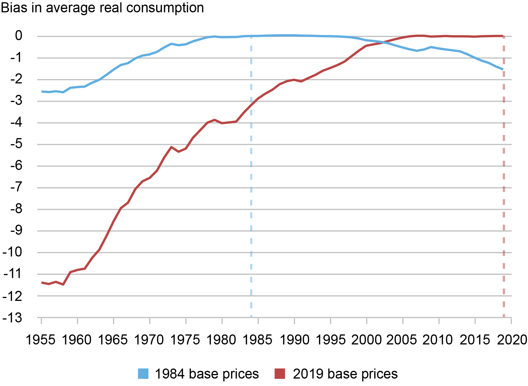
Source: Author’s calculations based on the historical linked CEX-CPI data.
Notes: This chart reports the biases in the level of average real consumption per household in conventional measures of real consumption, when compared against the corrections implied by our method, under two choices for the fixed prices as the base for calculation of real consumption: prices in 1984 and in 2019.
Of course, bias in measuring the level of real consumption leads to corresponding biases in the estimated growth. As the chart above already indicates, if we fix prices in the most recent year (2019), the conventional estimates overestimate the rate of growth in average real consumption due to the negative bias in the levels. In particular, the uncorrected measure of cumulative real consumption growth is 270 percent over the entire 1955-2019 period, or 2.07 percent growth annually. In contrast, with our correction for income dependence and under 2019 base prices, cumulative consumption growth falls to 232 percent, or an annualized growth rate of 1.89 percent per year. Thus, in this case we find that the annual growth rate from 1955 to 2019 is lowered by 18 basis points (2.07 percent − 1.89 percent).
Note that, since the conventional measure always underestimates the level of real consumption, the sign of the error in measured growth of real consumption depends on the choice of the base prices. For instance, if we instead fix 1984 prices as our base, the chart shows that the conventional measures in fact underestimate the growth in real consumption between 1984 and 2019. In other words, since preferences are income-dependent, measured growth in real consumption should in principle depend on the choice of fixed prices to express the measure.
Finally, we also apply our generalized method to quantify the adjustment to average real consumption implied by consumer aging in the United States. In this case, we reconstruct our measures of inflation by deciles of age and income by, first, defining ten deciles of the (pretax) income and, then, computing ten age deciles within each income decile. Using this data, as the chart below illustrates, we document a strong positive relationship between consumer age and inflation, which alters the measurement of real consumption because the average consumer age increases over time. We find that the implied adjustments to real consumption are economically meaningful but much smaller than the correction due to income dependence, which justifies our focus on the latter.
Consumer Aging and Real Consumption (1955-2019)
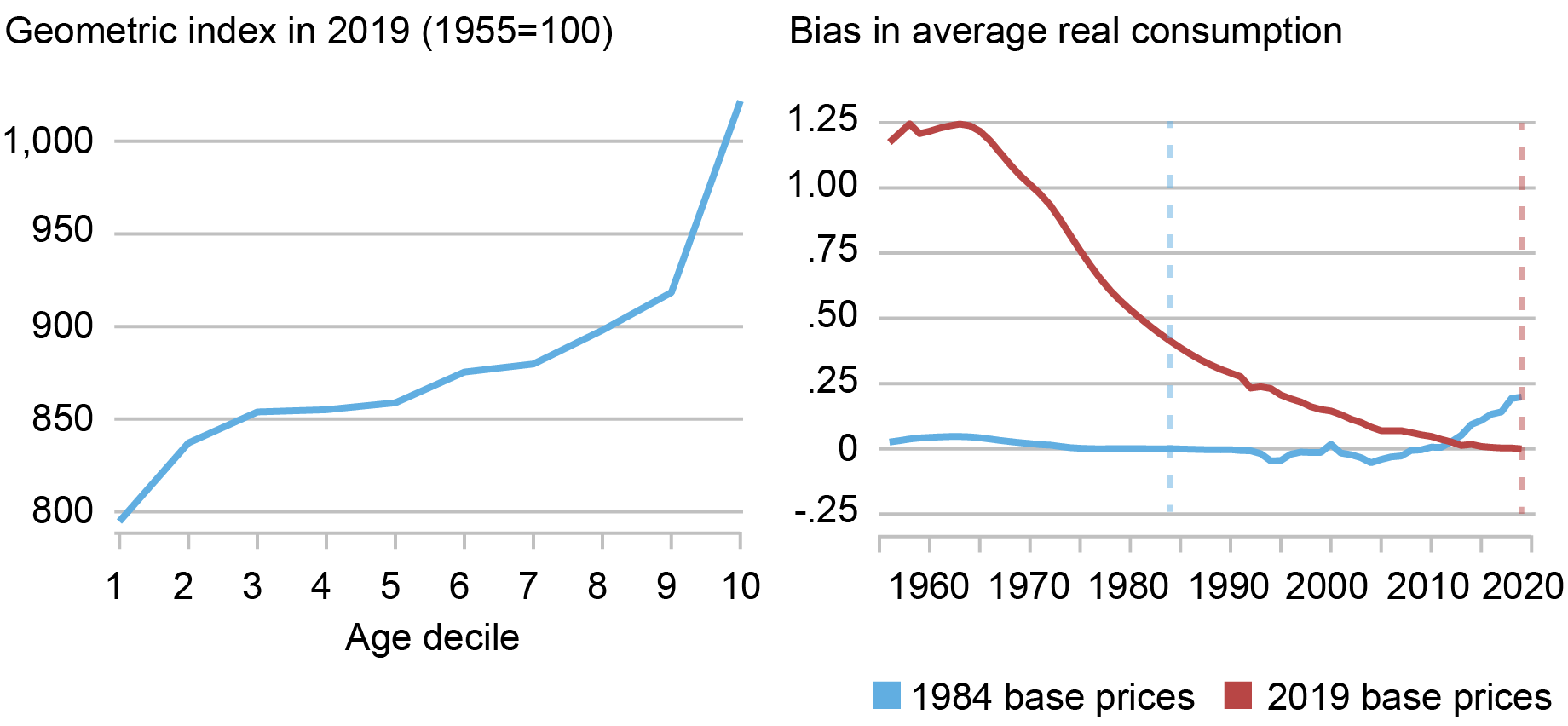
Sources: Author’s calculations based on the historical linked CEX-CPI data.
Notes: The left panel of the chart reports the cumulative inflation in the United States, from 1955 to 2019, for each decile of age. The right panel reports the implied bias in the average level of real consumption per household in conventional measures of real consumption, when compared against the corrections implied by our method due to aging, under two choices for the fixed prices as the base for calculation of real consumption: prices in 1984 and in 2019.
Conclusion
Our results may have important implications for the way in which national statistical agencies around the world construct measures of inflation and real economic value. In particular, the empirical results presented above suggest an approach that the Bureau of Labor Statistics (BLS) can use, based on already available data, to construct improved measures of real consumption growth and inequality in the U.S. In addition to improving the measurement of long-run growth and inflation inequality, our new approach can have important policy implications, such as the indexation of the poverty line and a more efficient targeting of welfare benefits. This approach also provides a blueprint for distributional national accounts (Piketty et al. 2018) that account for inflation inequality and income dependence in household preferences.

Danial Lashkari is a research economist in Labor and Product Market Studies in the Federal Reserve Bank of New York’s Research and Statistics Group.
How to cite this post:
Danial Lashkari, “Measuring Price Inflation and Growth in Economic Well‑Being with Income‑Dependent Preferences,” Federal Reserve Bank of New York Liberty Street Economics, January 8, 2024, https://libertystreeteconomics.newyorkfed.org/2024/01/measuring-price-in....
Was the 2021-22 Rise in Inflation Equitable?
Inflation Disparities by Race and Income Narrow
Disclaimer
The views expressed in this post are those of the author(s) and do not necessarily reflect the position of the Federal Reserve Bank of New York or the Federal Reserve System. Any errors or omissions are the responsibility of the author(s).
The magnificent failure of mainstream economics
The magnificent failure of mainstream economics Steve Keen For the last fifty years, the development of economics has been driven by the desire to derive…
The New York Fed DSGE Model Forecast—December 2023

This post presents an update of the economic forecasts generated by the Federal Reserve Bank of New York’s dynamic stochastic general equilibrium (DSGE) model. We describe very briefly our forecast and its change since September 2023. As usual, we wish to remind our readers that the DSGE model forecast is not an official New York Fed forecast, but only an input to the Research staff’s overall forecasting process. For more information about the model and variables discussed here, see our DSGE model Q & A.
The New York Fed model forecasts use data released through 2023:Q3, augmented for 2023:Q4 with the median forecasts for real GDP growth and core PCE inflation from the November release of the Philadelphia Fed Survey of Professional Forecasters, as well as the yields on 10-year Treasury securities and Baa-rated corporate bonds based on 2023:Q3 averages up to November 21. Starting in 2021:Q4, the expected federal funds rate (FFR) between one and six quarters into the future is restricted to equal the corresponding median point forecast from the latest available Survey of Primary Dealers (SPD) in the corresponding quarter. For the current projection, this is the November SPD.
The economy turned out to be stronger in Q3 than predicted by the model. This forecast error naturally pushes up the output growth forecast for the current year but has only a small impact on projections for activity otherwise. The model expects output growth to be 0.7 percentage points higher in 2023 than forecasted in September (2.6 versus 1.9 percent) but not very different from the September predictions for the rest of the forecast horizon (1.2, 0.7, and 0.9 percent in 2024, 2025, and 2026, versus 1.1, 0.7, and 1.2 percent in September, respectively). The output gap is projected to be somewhat lower in 2023 than was predicted in September, as the model attributes the recent strength of the economy mainly to supply rather than demand factors. The output gap predictions are similar to those made in September for the remainder of the forecast horizon. Inflation projections are lower in 2023 than they were in September (3.4 versus 3.7 percent), mostly because Q3 inflation surprised the model on the downside. The expected path for inflation is unchanged otherwise: 2.2 percent in 2024 and 2.0 percent in 2025 and 2026.
The short-run real natural rate of interest is expected to remain at the same elevated level as projected in September for 2023 (2.5 percent), declining to 2.2 percent in 2024, 1.8 percent in 2025, and 1.6 percent in 2026. The expected path of the policy rate is essentially unchanged relative to September. The model sees monetary policy as being restrictive through the end of 2024 in the sense that the FFR in real terms is above the short-term natural rate of interest.
Forecast Comparison
Forecast Period2023202420252026Date of ForecastDec 23Sep 23Dec 23Sep 23Dec 23Sep 23Dec 23Sep 23GDP growth
(Q4/Q4)2.6
(2.2, 3.0) 1.9
(0.2, 3.6) 1.2
(-3.8, 6.2) 1.1
(-4.0, 6.3) 0.7
(-4.3, 5.7) 0.7
(-4.4, 5.8) 0.9
(-4.5, 6.3) 1.2
(-4.2, 6.6) Core PCE inflation
(Q4/Q4)3.4
(3.3, 3.5) 3.7
(3.4, 3.9) 2.2
(1.5, 2.9) 2.2
(1.5, 3.0) 2.0
(1.1, 2.9) 2.0
(1.1, 2.9) 2.0
(1.0, 3.0) 2.0
(1.0, 3.0) Real natural rate of interest
(Q4)2.5
(1.4, 3.5) 2.5
(1.3, 3.7) 2.2
(0.8, 3.6) 2.2
(0.8, 3.7) 1.8
(0.3, 3.3) 1.9
(0.3, 3.4) 1.6
(0.0, 3.2) 1.6
(0.0, 3.3) Source: Authors’ calculations.
Notes: This table lists the forecasts of output growth, core PCE inflation, and the real natural rate of interest from the December 2023 and September 2023 forecasts. The numbers outside parentheses are the mean forecasts, and the numbers in parentheses are the 68 percent bands.
Forecasts of Output Growth
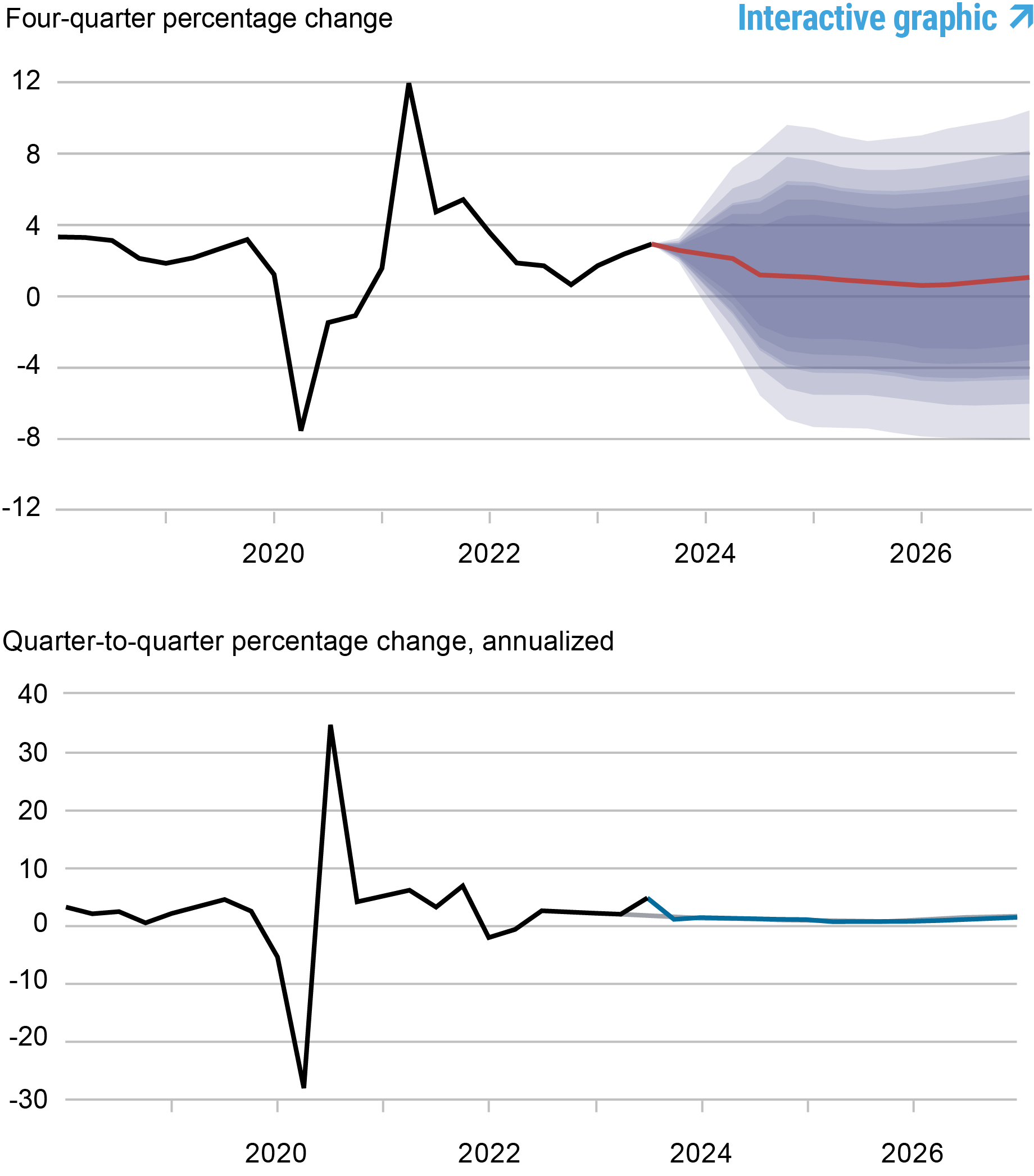 Source: Authors’ calculations.
Notes: These two panels depict output growth. In the top panel, the black line indicates actual data and the red line shows the model forecasts. The shaded areas mark the uncertainty associated with our forecasts at 50, 60, 70, 80, and 90 percent probability intervals. In the bottom panel, the blue line shows the current forecast (quarter-to-quarter, annualized), and the gray line shows the September 2023 forecast.
Forecasts of Inflation
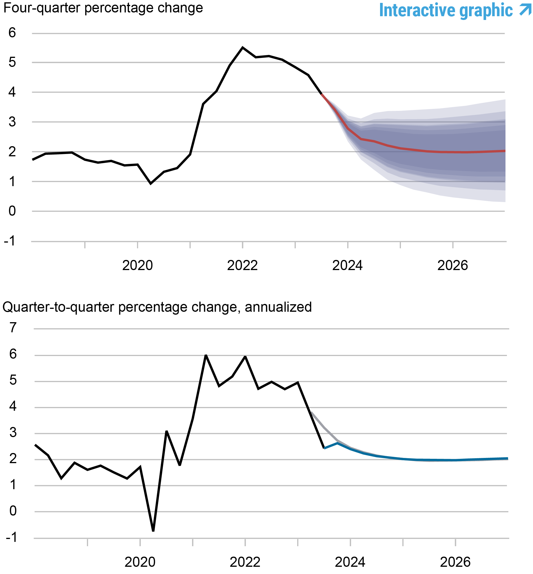 Source: Authors’ calculations.
Notes: These two panels depict core personal consumption expenditures (PCE) inflation. In the top panel, the black line indicates actual data and the red line shows the model forecasts. The shaded areas mark the uncertainty associated with our forecasts at 50, 60, 70, 80, and 90 percent probability intervals. In the bottom panel, the blue line shows the current forecast (quarter-to-quarter, annualized), and the gray line shows the September 2023 forecast.
Real Natural Rate of Interest
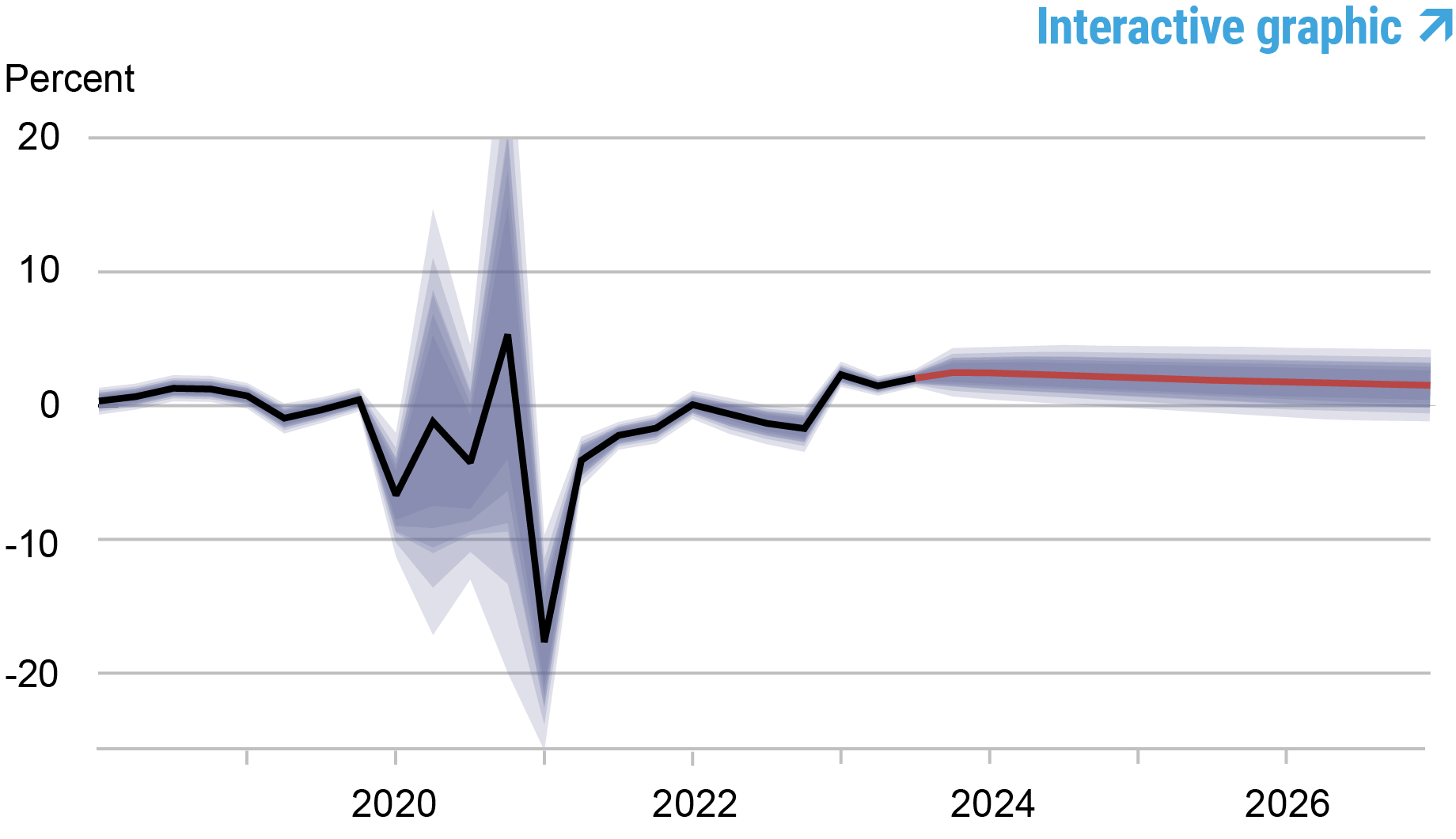 Source: Authors’ calculations.
Notes: The black line shows the model’s mean estimate of the real natural rate of interest; the red line shows the model forecast of the real natural rate. The shaded area marks the uncertainty associated with the forecasts at 50, 60, 70, 80, and 90 percent probability intervals.

Marco Del Negro is an economic research advisor in Macroeconomic and Monetary Studies in the Federal Reserve Bank of New York’s Research and Statistics Group.

Pranay Gundam is a research analyst in the Federal Reserve Bank of New York’s Research and Statistics Group.

Donggyu Lee is a research economist in Macroeconomic and Monetary Studies in the Federal Reserve Bank of New York’s Research and Statistics Group.

Ramya Nallamotu is a senior research analyst in the Federal Reserve Bank of New York’s Research and Statistics Group.

Brian Pacula is a research analyst in the Federal Reserve Bank of New York’s Research and Statistics Group.
How to cite this post:
Marco Del Negro, Pranay Gundam, Donggyu Lee, Ramya Nallamotu, and Brian Pacula, “The New York Fed DSGE Model Forecast—December 2023,” Federal Reserve Bank of New York Liberty Street Economics, December 15, 2023, https://libertystreeteconomics.newyorkfed.org/2023/12/the-new-york-fed-d....

The New York Fed DSGE Model Perspective on the Lagged Effect of Monetary Policy

The New York Fed DSGE Model Forecast— September 2023

The Evolution of Short-Run r* after the Pandemic
Disclaimer
The views expressed in this post are those of the author(s) and do not necessarily reflect the position of the Federal Reserve Bank of New York or the Federal Reserve System. Any errors or omissions are the responsibility of the author(s).
Why lower house prices could lead to higher mortgage rates
Fergus Cumming and Danny Walker

Bank Rate has risen by more than 5 percentage points in the UK over the past couple of years. This has led to much higher mortgage rates for many people. In this post we analyse another potential source of pressure on mortgagors: the potential for falls in house prices to push borrowers into higher – and therefore more expensive – loan to value (LTV) bands. In a scenario where house prices fall by 10% and high LTV spreads rise by 100 basis points, we estimate that an additional 350,000 mortgagors could be pushed above an LTV of 75%, which could increase their annual repayments by an extra £2,000 on average. This could have a material impact on the economy.
There is significant public and media attention on how the Bank of England’s interest rate decisions affect mortgagors. The interest rates set by central banks are of course a key determinant of the rates people pay on their mortgages. Banks tend to price mortgages off interest rate swaps, which reflect the market’s expectations of future policy rates. The relevant swap rates for the 80% of UK mortgages that have fixed interest rates are typically the two and five-year rates. While Bank Rate has risen by more than 5 percentage points since December 2021, the two-year swap rate has risen by 4.6 percentage points and two-year mortgage rates have risen by around 4.5 percentage points (Chart 1). But Bank Rate is not the only determinant of mortgage rates.
Chart 1: Mortgage rates have increased sharply in the UK – they tend to be priced off swap rates, which are linked to Bank Rate

Note: The chart shows quoted rates for two-year mortgages at different LTV ratio bands. It compares them to Bank Rate (the Bank of England policy rate) and the two-year swap rate, both of which are considered risk-free rates.
Source: Bank of England.
Mortgages with lower deposits – higher LTV ratios – have higher interest rates, but the spread is currently very low
Loosely speaking, a mortgage interest rate is made up of the risk-free rate – typically the relevant swap rate – and some compensation for risk, known as the spread. LTV ratios are the key determinant of spreads. For example, someone with a deposit of at least 25% of the value of the house at the point the mortgage is issued qualifies for a 75% LTV mortgage, which comes with a lower interest rate than if they only had a deposit worth 10% of the value. Mortgages with higher deposits, and therefore lower LTVs, are generally safer for banks because higher deposits means borrowers can withstand larger house price falls before falling into negative equity. Higher LTV mortgages tend to have higher interest rates for that reason.
Throughout the 2010s it was common for the spread between 90% and 75% LTV mortgage rates to be between 1 and 2 percentage points (Chart 1). As of August 2023, that spread was less than 0.4 percentage points. In fact, spreads have been very narrow since 2021 and the last time spreads were at today’s levels was probably in 2008, which is before the official data began. Given that high LTV mortgages look relatively cheap compared with recent history, we construct an illustrative scenario where the 90% LTV spread returns to close to its post-2010 average – something we regard as plausible.
We analyse an illustrative scenario where mortgage spreads rise by 100 basis points and house prices fall by 10% from their peak
Our aim is not to forecast what will happen in the mortgage market, but simply to examine a set of conditions that are within the realms of possibility. We use data on the universe of UK owner-occupier mortgages in the Product Sales Database. The most detailed information is recorded when mortgages are originated for the first time and upon remortgage. We build a snapshot of the mortgage market by modelling how much principal people have paid down since origination and how house prices have evolved in their region. We focus on mortgages originated since 2020 Q4 because they are most likely to have high LTV ratios, given the borrowers have not had much time to pay down principal and have had less time to benefit from significant house price increases.
In our scenario analysis, the 90% LTV mortgage rate increases by 100 basis points (Chart 2) and house prices fall by 10% (Chart 3). As a comparison, in the 2007 to 2009 financial crisis, the 90% LTV spread – measured versus 60% LTV mortgages – reached over 250 basis points and house prices fell by almost 20% from peak to trough.
Chart 2: In our scenario analysis, the interest rates on mortgages with LTV ratios of above 75% increase by 100 basis points, taking them closer to historical spreads

Note: The chart shows quoted rates for two-year mortgages at different LTV bands, expressed as a spread versus the 0%–60% LTV rate. We analyse an indicative scenario where the spread on 75%–90%, 90%–100% and 100%+ LTV mortgages rises by 100 basis points.
Source: Bank of England.
We recalculate LTVs following the 10% fall in house prices in the scenario and assume all mortgagors eventually have to refinance at the new higher rate for their LTV band. In the real world, mortgagors reaching the end of their fixed term will face a recalculation of their LTV based on a revaluation of their house, which is typically calculated using private sector indices. As it happens, those indices have already fallen by a few per cent more than the official price index shown on Chart 3. We do not model mortgage choice in the scenario: for simplicity we assume that mortgagors take out a two-year fixed-rate mortgage.
Chart 3: In our scenario analysis, UK average house prices fall by 10%, taking them back to around their 2021 level

Note: The chart shows the UK house price index expressed as a percentage change since the start of 2010. We analyse an indicative scenario where the index falls by 10%.
Sources: Bank of England and Office for National Statistics.
The scenario pushes an additional 350,000 mortgagors above 75% LTV, increasing their annual repayments by £2,000 on average
At origination, around 40% of recent mortgages had deposits that were too small to be eligible for a 0%–60% or 60%–75% LTV mortgage. When we take account of principal repayments and house price growth since origination, that suggests around a quarter of recent mortgages – just under 800,000 – are above that 75% LTV threshold now.
We find that the house price fall in our scenario pushes an additional 350,000 mortgagors above the 75% LTV threshold, taking the total back to around 40% of recent mortgagors (Chart 4), or 1.1 million. It also pushes around 3% into negative equity. The assumed 100 basis point increase in mortgage spreads in the scenario leads to an average increase in annual repayments for these mortgagors of just over £2,000 by the time they refinance, over and above the impact from the increase in swap-rates. That is clearly a material impact for the people affected, but is it material for the economy?
Chart 4: The scenario leads to a rise in LTV ratios for recent mortgagors, which comes with higher interest rates

Note: The chart shows all UK owner-occupier mortgages in the Product Sales Database originated since 2020 Q4, split by LTV ratio. We update the loan amount outstanding by modelling the scheduled flow of principal repayments for each loan. We update the house price based on an assumption that house prices have evolved in line with the average price in their region (eg London, South East of England etc). The scenario reduces prices uniformly by 10%. We assume for simplicity that there are no 80% LTV products. The numbers should be interpreted as indicative rather than a precise read on the stock of UK mortgages.
Sources: Bank of England and Financial Conduct Authority Product Sales Database.
The macro impact of this scenario could be material, given that it affects those mortgagors that are most financially constrained
At first glance, the impact of this scenario looks relatively modest in comparison to the increase in Bank Rate that has already occurred. The 100 basis point increase in mortgage spreads in our scenario is less than a quarter of the size of the rise in swap rates that has already occurred. It also only affects 40% of recent mortgagors, and just over 10% of all mortgagors. Focusing on recent mortgagors, our analysis suggests that their aggregate additional repayment burden (£2.4 billion) amounts to around 20% of the total repayment increase caused by the rise in Bank rate on its own (£11 billion).
But it is also true that the mortgagors impacted by this scenario are some of the most financially constrained households, and some of the most important for policymakers to consider. Well-established theoretical research has emphasised the role of heterogeneity in macroeconomics and empirical research has previously explored the importance of the most levered mortgagors in the transmission of monetary policy. To the extent that the scenario affects households most likely to substantially change their spending patterns, it is plausible that this amplification channel is not trivial. Indeed, for the most levered mortgagors, the scenario eventually increases repayments by 40% over-and-above the rise in mortgage rates already baked in.
Implications
Policymakers across the globe are well versed in the importance of the housing and mortgage markets, particularly for monetary policy transmission. The financial crisis is still in the rear-view mirror and much has been learned from it. But this post highlights an interesting channel of monetary policy which, while it will be captured implicitly in some models, is often less discussed outside policy circles. The scenario analysis reminds us that there can be more to monetary policy tightening than risk-free rates. Many people expect the tightening that has already occurred to lead to a significant fall in house prices, and it is plausible that mortgage spreads will return to historical levels. Although there is uncertainty, this has the potential to lead to a material impact on economic activity over and above the impact of risk-free rates.
Fergus Cumming is Deputy Chief Economist at the Foreign, Commonwealth and Development Office. He used to work on monetary policy and financial stability at the Bank. Danny Walker works in the Bank’s Deputy Governor’s office.
If you want to get in touch, please email us at bankunderground@bankofengland.co.uk or leave a comment below.
Comments will only appear once approved by a moderator, and are only published where a full name is supplied. Bank Underground is a blog for Bank of England staff to share views that challenge – or support – prevailing policy orthodoxies. The views expressed here are those of the authors, and are not necessarily those of the Bank of England, or its policy committees.
Added to Provisioning & Prosperity
Much of Microeconomics: Provisioning & Prosperity concerns local alternative/complimentary currencies. I began looking for reports or commentary to learn about the impacts on the participating organizations and agencies. Those who used — but did not issue — the currencies.
What I’ve found offer detailed descriptions of operations, student responses, lessons learned, types of organizational participants, etc. All important to know, but, readers familiar with impact/output evaluation models may notice what’s missing. They make little or no mention of the impact of using these local currencies to employ students had on the agencies that took advantage of the programs.
Stay tuned. Meanwhile,
here are the latest additions to Microeconomics: Provisioning & Prosperity”
Currency, coercion and campuses
— Alan Hutchison Matches in the Dark· Nov 20, 2020 (updated)
The Paper Chase
— Rob Trump The New Inquiry April 25, 2014
The Buckaroo and the Demand for Money
— John Carney (@Carney) CNBC Feb 9, 2012
The UMKC Buckaroo- A Currency Model for World Prosperity
— Warren Mosler (@WBMosler) MoslerEconomics/Modern Monetary Theory Nov 20, 2011
BerkShares, Buckaroos, and Bear Dollars: What Makes a Local Currency Tick?
— L. Randall Wray New Economic Perspectives July 13, 2009
Time for a Sterling Crisis?
The UK pound plunged again earlier this month:

two dates are marked with vertical lines: the the Brexit vote (red line) and the Prime Minister's speech signalling that the most likely outcome was a "hard Brexit" (green line) where the UK leaves the European single market (i.e., that it won't become part of the European Economic Area, like Finland* Norway, or negotiate an arrangement like Switzerland's).
Departure from the EU and the single market make the UK a less attractive location for foreign investment (see, e.g., comments from Nissan's CEO about its Sunderland plant). A decrease in demand for UK assets implies a drop in the pound. The UK is also a less attractive location for domestic investment now as well, and the situation is probably not a good one for consumer confidence - a reduction in demand due to lower desired consumption and investment would imply lower interest rates, which also would cause the pound to fall.
Is this yet another "sterling crisis"? Not in the usual sense - as Gavyn Davies notes, there is no fixed exchange rate to defend this time, and most of the UK's external debt is denominated in pounds.
As Paul Krugman explains, a fall in the pound is a part of the adjustment process. He writes:
But it’s important to be aware that not everyone in Britain is equally affected. Pre-Brexit, Britain was obviously experiencing a version of the so-called Dutch disease.
In its traditional form, this referred to the way natural resource
exports crowd out manufacturing by keeping the currency strong. In the
UK case, the City’s financial exports play the same role. So their
weakening helps British manufacturing – and, maybe, the incomes of
people who live far from the City and still depend directly or
indirectly on manufacturing for their incomes.
However, a rebalancing of the UK economy in favor of manufacturing exports will not come quickly, according to Barry Eichengreen (Robert Skidelsky goes further and argues for helping the process along through "import substitution" policies).
One likely consequence is inflation, as Ambrose Evans-Pritchard writes. Prices of imported goods will rise significantly (though the process of "exchange rate pass-through" generally occurs with a lag - the "marmite row" may have been a harbinger of things to come). The inflation will hit lower-income families especially hard, according to Evans-Pritchard's column, because the government has frozen some benefit payments, so inflation will cause their real value to fall.
Rising costs for imports don't only impact consumers - they also affect producers. On the one hand, domestic producers benefit from increases in the relative prices of imported substitutes. On the other - and this is becoming more and more relevant in an age of global supply chains - prices of imported inputs (intermediate goods) will rise, increasing production costs.
With the rise in cost of intermediate inputs and the greater costs of selling to its main trading partners, the impact of Brexit looks like a negative supply shock. Supply shocks create a nasty dilemma for monetary policy. Policy can "accommodate" the shock by allowing inflation to rise - doing so minimizes the increase in unemployment and helps keep output near its (diminished) potential. Or the Bank of England could tighten policy to keep inflation in check, with negative consequences for output and employment.
The risk with accommodation is not just inflation itself, but a potential increase in inflation expectations and loss of the central bank's credibility. Part of the standard interpretation of 1970's stagflation is that the Fed was too accommodating after the 1973 oil shock, and which contributed to inflation expectations getting out of control.
The Bank of England has a formal 2% inflation target; right now inflation is running below target, but that will change.

I personally think its to Bank of England's credit that it's allowed inflation go above target at a couple of points during the turmoil of recent years. If their policy is credible, an occasional miss doesn't cause inflation expectations to rise. But the point of inflation targeting is to achieve credibility by meeting a stated target, so the BofE may be putting that at risk if it's always seen to be accommodating shocks.
*corrected 10/26
Lies, Damned Lies and Ireland's GDP
Being an academic economist can be humbling - while it involves learning lots of esoteric stuff, it also makes one much more aware of how much one doesn't know. But I know this much is true: the total amount of goods and services produced in Ireland did not increase by 26.3% in 2015.
But that's what Ireland's Central Statistics Office has reported. It's not entirely clear how they came to such a (literally) incredible figure for real GDP growth. The expenditure approach to calculating GDP adds up purchases of new final goods and services in four categories - consumption (C), investment (I), government purchases (G) and net exports (NX). I took the data from table 6 of their release and normalized each component to 100 in 2010 to illustrate how the change is driven by large jumps in I and NX.

News reports have focused on activities of multinational corporations, particularly on "inversions" which involve transferring their legal headquarters to Ireland in order to take advantage of its low corporate tax rates.
That may be correct, but its not an entirely satisfying explanation. GDP is supposed to measure the value of goods and services produced in a country. The legal domicile of the corporations producing it is irrelevant. Ownership of capital - both physical machinery, equipment and structures and also intangible forms (intellectual property, etc.) - also is irrelevant, so the fact that multinational corporations like to hold IP in Ireland for tax reasons shouldn't matter in principle.
Gross National Product (GNP) adds up the total value of goods and services produced with resources owned by a country's citizens. Since many multinational corporations operate in Ireland, it has higher GDP than GNP because some of its GDP is produced using foreign-owned capital - the same data release showed a shocking increase of 18.7% in Ireland's GNP last year.
The information released by the CSO is not very detailed. The FT Alphaville's Matthew Klein, Bloomberg Columnist Leonid Bershidsky, and Seamus Coffey at the Irish Economy blog have made useful attempts at sorting things out.
Clearly, the way the CSO is calculating GDP is failing to correspond to the concept. Statistical agencies need to provide estimates calculated in a consistent fashion, so it wouldn't have been appropriate for them to suddenly decide to calculate it differently because they got a strange number. But the methods for estimating GDP are not etched in stone. If legal and accounting maneuvers of multinationals are distorting some of their source data, they need to find a way of correcting for it. Standards for national accounts are coordinated internationally and it is not clear whether the problems in this report are due to something the CSO is doing or a more general methodological issue which happens to be most apparent because of Ireland's unique circumstances.
Statistical agencies update their methods and revise their estimates regularly - e.g., in 2013, the US BEA did a "comprehensive revision" that began the treatment of development of intellectual property as a component of investment (see this earlier blog post). I hope the CSO will release more information to help everyone better understand what's gone wrong with their figures. That will be a first step towards correcting the method used to estimate GDP and producing a revised set of figures - one which will not show a 26% increase in real GDP in 2015.
Update: Procedures mandated by Eurostat are mostly to blame, writes Colm McCarthy.
Hysteresis in a New Keynesian Model
I've posted a draft of my research paper, "Hysteresis in a New Keynesian Model" on my website. The paper proposes a way of modelling hysteresis and integrates it into a New Keynesian macro model.
The widely noted rightward shift of the Beveridge curve relationship can be interpreted as evidence of less efficient matching between employers and workers in the labor market

In the paper, I argue that less-efficient matching is related to the increased duration of unemployment spells seen during the last recession and its aftermath. There are several reasons why matching may be less efficient with a higher proportion of long-term unemployed:
- a loss of information as workers' informal networks may dry up over time
- a stigma associated with long-term unemployment (i.e., it acts as a negative signal)
- decreased search effort by long-term unemployed
I cite empirical evidence for (2) and (3) in the paper. The paper does not take a stand on the mechanism causing the relationship between matching efficiency and duration of unemployment.
The model includes a Diamond-Mortensen-Pissarides search-and-matching labor market framework, where hires (H) are a function of the number of vacancies (V) posted by firms and unemployed (U) workers

Hysteresis is modeled with the assumption that matching efficiency (A) is a decreasing function of the average duration of unemployment spells.
Rearranging the matching function to solve for efficiency (and setting alpha to 0.5), we can see that a decrease in efficiency coincides with the increase in the duration of unemployment spells

With hysteresis, the response of unemployment to a negative productivity shock is smaller initially but more persistent, as shown by the impulse response functions:

The reason for this is that, in the absence of hysteresis, firms can adjust their labor by sharply decreasing their vacancy posting. With hysteresis, the response of vacancies is less dramatic because firms take into account the fact that hiring will be more difficult in the future due to the decline in matching efficiency.
The model also considers demand shocks, which take the form of shocks to the discount factor, and monetary shocks (deviations from the Taylor rule), with similar results. Overall, hysteresis acts as a mechanism that increases the persistence of the response of macroeconomic variables to shocks. Since macro models struggle to generate endogenous persistence, this may be one of the main selling points of the paper.
Hysteresis also generates movements in the "natural rate" of unemployment, which I proxy by computing the amount of unemployment that would occur if wages and prices were flexible, taking as given the evolution of matching efficiency (A) from the baseline model. The green line shows the change in the natural rate in response to a negative productivity shock:

Note: this is a revised version of the draft circulated last fall as my "job market paper".
Productivity Pessimism
I'm hoping I'll have a chance to read Robert Gordon's new book soon, though one of the ironies of being a college professor is that the job doesn't seem to leave much time to read. Fortunately, Gordon presents a condensed version of the argument in a recent Bloomberg View column, where he explains that he doesn't expect a return to the rapid productivity growth of the mid-20th century. He writes:
The 1920-70 expansion grew out of the second industrial revolution, when
fossil fuels, the internal-combustion engine, advanced metals and
factory automation came together to produce electric lighting, indoor
plumbing, home appliances, motor vehicles, air travel, air conditioning,
television and much longer life expectancy.
The "third industrial revolution" - computers and the internet - is less significant, in his view:
Although revolutionary, the Internet's effects were limited when
compared with the second industrial revolution, which changed
everything. The former had little effect on purchases of food, clothing,
cars, furniture, fuel and appliances. A pedicure is a pedicure whether
the customer is reading a magazine or surfing the web on a smartphone.
Computers aren't everywhere: We don’t eat, wear or drive them to work.
We don't let them cut our hair. We live in dwellings that have
appliances much like those of the 1950s and we drive in motor vehicles
that perform the same functions as in the 1950s, albeit with more
convenience and safety.
Our main measure of technological progress is total factor productivity (tfp) growth, which is sometimes called the "Solow residual" because it is calculated as a leftover, by subtracting from output growth the portions that can be explained by changes in capital and labor. That is, it is the growth that would occur even if there was no change in the factors of production.
Turning points in tfp growth can be hard to identify because the data are somewhat volatile from year-to-year and have a cyclical component. With hindsight, economists identified a productivity slowdown around 1973 and a resurgence - with information technology playing a leading role - in the mid-1990s. However, tfp growth has generally been weak since 2005, raising the question of whether the IT-led productivity boom is over.

Data: Bureau of Labor Statistics
This San Francisco Fed Letter from last year discusses some of the reasons for the productivity slowdown. Gordon's book was the subject of an Eduardo Porter column and a Paul Krugman review.
Update (2/25): In an interview with Ezra Klein, Bill Gates argues against Gordon's view.