macroeconomics
Has Market Concentration in U.S. Manufacturing Increased?

The increasing dominance of large firms in the United States has raised concerns about pricing power in the product market. The worry is that large firms, facing fewer competitors, could increase their markups over marginal costs without fear of losing market share. In a recently published paper, we show that although sales of domestic firms have become more concentrated in the manufacturing sector, this development has been accompanied by the entry and growth of foreign firms. Import competition has lowered U.S. producers’ share of the U.S. market and put smaller, less efficient domestic firms out of business. Overall, market concentration in manufacturing was stable in recent decades, though import penetration has greatly altered the makeup of the U.S. manufacturing sector.
Measuring Concentration
Many previous studies have focused on what we refer to as production concentration, which is measured as the sales of the largest U.S. producers as a share of total production in the U.S. That is, it does not take account of imported goods, but does include U.S. firms’ exports. As shown in the charts below, the production concentration of the top-four or top-twenty firms has increased between 1992 and 2012 (blue lines). For questions related to market power in the labor market, the evolution of production concentration is indeed relevant. However, for questions related to market power in the product market, we need to take into account the sales of foreign exporters in the United States (and exclude U.S. firms’ sales abroad). We refer to this measure of concentration as market concentration. The chart below shows that the largest firms’ (which could be U.S. or foreign) share of total sales (inclusive of sales by foreign firms) in U.S. manufacturing industries has been flat in the aggregate (red lines). The construction of market concentration, using the full sales distribution, was only made possible by accessing confidential census data, which report the sales in the U.S. of both domestic firms and foreign exporters.
U.S. Production Concentration Has Risen, but Overall Market Concentration Has Remained Flat
Top-4 market share
{"padding":{"auto":false,"bottom":0,"right":0,"left":33},"axis":{"rotated":false,"x":{"show":true,"type":"category","localtime":true,"tick":{"centered":false,"culling":false,"fit":true,"outer":true,"multiline":false,"multilineMax":0},"label":{"text":"","position":"outer-center"},"categories":["1992","1997","2002","2007","2012"]},"y":{"show":true,"inner":false,"type":"linear","inverted":false,"tick":{"centered":false,"culling":false,"values":["0.4","0.3","0.2","0.35","0.25"]},"padding":{"top":3,"bottom":0},"primary":"","secondary":"","label":{"text":"","position":"outer-middle"},"max":0.4,"min":0.2},"y2":{"show":false,"inner":false,"type":"linear","inverted":false,"padding":{"top":3},"label":{"text":"","position":"outer-middle"}}},"chartLabel":"Top-4 market share","color":{"pattern":["#61AEE1","#B84645","#B1812C","#046C9D","#9FA1A8","#DCB56E"]},"interaction":{"enabled":true},"point":{"show":false},"data":{"groups":[],"labels":false,"type":"line","order":"desc","selection":{"enabled":false,"grouped":true,"multiple":true,"draggable":true},"x":"","rows":[["Production concentration","Market concentration"],["0.34","0.31"],["0.35","0.3"],["0.37","0.31"],["0.37","0.3"],["0.38","0.3"]]},"legend":{"show":true,"position":"bottom"},"tooltip":{"show":true,"grouped":true},"grid":{"x":{"show":false,"lines":[],"type":"indexed","stroke":""},"y":{"show":true,"lines":[],"type":"linear","stroke":""}},"regions":[],"zoom":false,"subchart":false,"download":true,"downloadText":"Download chart","downloadName":"chart","trend":{"show":false,"label":"Trend"}}
Top-20 market share
{"padding":{"auto":false,"left":33,"right":0},"axis":{"rotated":false,"x":{"show":true,"type":"category","localtime":true,"tick":{"centered":false,"culling":false,"fit":true,"outer":true,"multiline":false,"multilineMax":0},"label":{"text":"","position":"outer-center"},"categories":["1992","1997","2002","2007","2012"]},"y":{"show":true,"inner":false,"type":"linear","inverted":false,"tick":{"centered":false,"culling":false,"values":["0.7","0.65","0.6","0.55","0.5"]},"padding":{"top":3,"bottom":0},"primary":"","secondary":"","label":{"text":"","position":"outer-middle"},"min":0.5,"max":0.7},"y2":{"show":false,"inner":false,"type":"linear","inverted":false,"padding":{"top":3},"label":{"text":"","position":"outer-middle"}}},"chartLabel":"Top-20 market share","color":{"pattern":["#61AEE1","#B84645","#B1812C","#046C9D","#9FA1A8","#DCB56E"]},"interaction":{"enabled":true},"point":{"show":false},"data":{"groups":[],"labels":false,"type":"line","order":"desc","selection":{"enabled":false,"grouped":true,"multiple":true,"draggable":true},"x":"","rows":[["Production concentration","Market concentration"],["0.600","0.544"],["0.610","0.539"],["0.630","0.544"],["0.640","0.535"],["0.650","0.539"]]},"legend":{"show":true,"position":"bottom"},"tooltip":{"show":true,"grouped":true},"grid":{"x":{"show":false,"lines":[],"type":"indexed","stroke":""},"y":{"show":true,"lines":[],"type":"linear","stroke":""}},"regions":[],"zoom":false,"subchart":false,"download":true,"downloadText":"Download chart","downloadName":"chart","trend":{"show":false,"label":"Trend"}}
Sources: U.S. Census Bureau; Amiti and Heise “U.S. Market Concentration and Import Competition,” Review of Economic Studies, April 2024.
Note: Concentration measures are simple averages across 169 industries at the five-digit North American Industry Classification (NAICS) level.
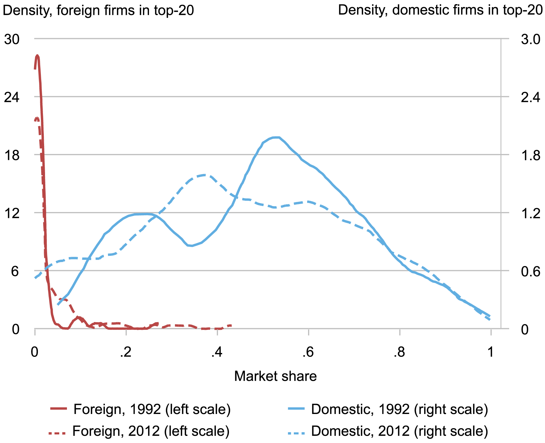
We illustrate the loss in U.S. firms’ market shares in the chart below, by plotting the distribution of the market shares of foreign firms (in red) and domestic firms (in blue) that are in the top-20 across industries in 1992 (solid lines) and in 2012 (dashed lines). To construct the graph, we take the top 20 firms in each industry, and identify among them the domestic and foreign firms. For any given market share, the height of the blue curve reflects the number of industries where the domestic firms have that market share, and analogously the red curve is for the foreign firms’ market shares.
Two main points stand out. First, the shift to the left of the blue line highlights the fall in the market share of domestic firms between 1992 and 2012. In the average industry, domestic firms in the top-20 had a market share of only about 40 percent in 2012 compared to 50 percent in 1992, which can be seen by comparing the peak of the curves.
Second, the shift to the right in the red line shows that foreign firms have gained some market share in the top-20 during our sample period: the share of industries where foreign firms in the top-20 have a near-zero market share has fallen, while the share of industries where foreign firms have a greater market share than 20 percent has risen. Despite this rise, it is important to note that in many industries the market share of foreign firms in the top-20 is still low: the aggregate market share of foreign firms in manufacturing sales is less than 4 percent in 2012. In our previous post, we showed that most of the foreign firms’ gains occurred at the bottom of the market share distribution.
Foreign Firms Have Gained Some Market Share in the Top 20
 Source: U.S. Census Bureau; Amiti and Heise “U.S. Market Concentration and Import Competition,” Review of Economic Studies, April 2024.
Notes: We exclude industries with no foreign firms in the top-20 from the foreign densities to zoom in on industries with a foreign firm presence. The number of industries with no foreign firms in the top-20 fell from one half to one third of all manufacturing industries during our sample period.
Is there a causal link between the rise in import competition and the concentration patterns we observe? Over the last few decades, U.S. manufacturing firms have become more exposed to foreign competition: import penetration (defined as the share of imports in domestic sales) has risen by about 10 percentage points between 1992 and 2012, from 10 percent to 20 percent. Our regression analysis shows that, in the average industry, a 10 percentage point increase in import penetration has caused a 2.1 percentage point rise in production concentration (see table below). Intuitively, an increase in import competition leads small, less efficient domestic firms to lose market share relative to larger, more efficient domestic firms. As a result, production concentration rises. We find that this effect is strongest in industries where goods are close substitutes.
Rising import penetration reduced the sales of U.S. firms as a share of the overall U.S. market (inclusive of foreign firms’ sales). However, this effect was nearly completely offset by the market share gains of foreign firms. Our estimates indicate that a 10 percentage point increase in import penetration increased the market share of foreign firms in the top-20 by 3.8 percentage points, while lowering the market share of domestic firms in the top-20 by 3.4 percentage points. As a result, market concentration remained virtually unchanged. We also find that rising import penetration has reduced the number of U.S. firms in manufacturing industries, as inefficient producers have been replaced by foreign firms.
Rising Import Penetration Caused Domestic Firms to Lose Market Share to Foreign Firms
Effect of a 10 Percentage Point Change in Import Penetration Production concentration +2.1** Market share of domestic firms in top-20 -3.4*** Market share of foreign firms in top-20 +3.8*** Market concentration +0.4 Number of domestic firms (percent) -23.0*** Source: U.S. Census Bureau.
Notes: The reported numbers are from regression tables in Amiti and Heise “U.S. Market Concentration and Import Competition,” Review of Economic Studies, April 2024. Three stars indicate significance at the 1 percent level; 2 stars indicate significance at the 5 percent level. All figures are percentage points unless otherwise specified.
In summary, our results show that import competition has contributed to increased production concentration due to a reallocation of market share from small domestic firms to large ones. At the same time, greater import competition reduced the overall market share of U.S. firms and increased that of foreign firms, resulting in stable market concentration. Interpreted through the lens of standard trade models, which imply a positive relationship between market shares and markups, our finding that U.S. firms’ market share has fallen suggests that the market power of U.S. manufacturing firms may actually have declined over the past few decades.

Mary Amiti is the head of Labor and Product Market Studies in the Federal Reserve Bank of New York’s Research and Statistics Group.

Sebastian Heise is a research economist in Labor and Product Market Studies in the Federal Reserve Bank of New York’s Research and Statistics Group.
How to cite this post:
Mary Amiti and Sebastian Heise, “Has Market Concentration in U.S. Manufacturing Increased? ,” Federal Reserve Bank of New York Liberty Street Economics, May 3, 2024, https://libertystreeteconomics.newyorkfed.org/2024/05/has-market-concent....

U.S. Market Concentration and Import Penetration

Global Supply Chains and U.S. Import Price Inflation

The Anatomy of Export Controls
Disclaimer
The views expressed in this post are those of the author(s) and do not necessarily reflect the position of the Federal Reserve Bank of New York or the Federal Reserve System. Any errors or omissions are the responsibility of the author(s).
MMT sees America through rapid economic recovery
MMT sees America through rapid economic recovery Stephanie Kelton and Steven Hail Modern monetary theory has been influential in helping America rise out of the…
Quantifying the macroeconomic impact of geopolitical risk
Julian Reynolds

Policymakers and market participants consistently cite geopolitical developments as a key risk to the global economy and financial system. But how can one quantify the potential macroeconomic effects of these developments? Applying local projections to a popular metric of geopolitical risk, I show that geopolitical risk weighs on GDP in the central case and increases the severity of adverse outcomes. This impact appears much larger in emerging market economies (EMEs) than advanced economies (AEs). Geopolitical risk also pushes up inflation in both central case and adverse outcomes, implying that macroeconomic policymakers have to trade-off stabilising output versus inflation. Finally, I show that geopolitical risk may transmit to output and inflation via trade and uncertainty channels.
How has the global geopolitical outlook evolved?
Risks from geopolitical tensions have become of increasing concern to policymakers and market participants this decade.
A popular metric to monitor these risks is the Geopolitical Risk (GPR) Index constructed by Caldara and Iacoviello (2022). The authors construct their index using automated text-search results from newspaper articles. Namely, they search for words relevant to their definition of geopolitical risk, such as ‘crisis’, ‘terrorism’ or ‘war’. They also construct GPR indices at a disaggregated country-specific level, based on joint occurrences of key words and specific countries.
Chart 1 plots the evolution of the geopolitical risks over time. Most notably, the Global GPR Index (black line) spikes following the 11 September attacks. More recently, this index shows a sharp increase following Russia’s invasion of Ukraine in February 2022.
Country-specific indices typically co-move significantly with the Global index but may deviate when country-specific risks arise. For instance, the UK-specific (aqua line) and France-specific indices (orange line) show more pronounced spikes following terrorist attacks in London and Paris respectively, while the Germany-specific index (purple line) rises particularly strongly following the invasion of Ukraine.
Chart 1: Global and country-specific Geopolitical Risk Indices

The GPR index is similar to the Economic Policy Uncertainty (EPU) index, produced by Baker, Bloom and Davis. The EPU index is also constructed based on a text search from newspaper articles, and available at both a global and country-specific level. But it measures more generic uncertainty related to economic policymaking, besides uncertainty stemming from geopolitical developments.
How to quantify the macroeconomic impact of these developments?
In light of increasing concerns about geopolitical tension, a growing body of literature aims to quantify the macro-financial impact of these developments. For instance, Aiyar et al (2023) examine multiple transmission channels of ‘geoeconomic fragmentation’ – a policy-driven reversal of global economic integration – including trade, capital flows and technology diffusion. Also Caldara and Iacoviello (2022) employ a range of empirical techniques to examine how shocks to their GPR affect macroeconomic variables.
These studies unambiguously show that geopolitical tension has adverse effects on macroeconomic activity and contributes to greater downside risks. But empirical estimates tend to differ significantly, depending on the nature and severity of scenarios through which geopolitical tensions may play out.
My approach focusses on the impact of geopolitical risks on a range of macroeconomic variables. Namely, I use local projections (Jordà (2005)), an econometric approach which examines how a given variable responds in the future to changes in geopolitical risk today. I employ a panel data set of AEs and EMEs (listed in Table A), with quarterly data from 1985 onwards.
Table A: List of economies

Notes: Countries divided into Advanced and Emerging Market Economies as per IMF classification. Country-level EPU indices available for starred economies.
Following Caldara and Iacoviello (2022), I regress a given variable on the country-level GPR index, controlling for: country-level fixed effects; the global GPR index; the first lag of my variable of interest; and the first lags of (four-quarter) GDP growth, consumer price inflation, oil price inflation, and changes in central bank policy rates.
I use ordinary least squares estimation to estimate the mean response over time of a given macroeconomic variable to geopolitical risk. But to assess the impact of geopolitical risk at the tail of the distribution, I follow Lloyd et al (2021) and Garofalo et al (2023) by using local-projection quantile regression. This latter approach uses an outlook-at-risk framework to illustrate how severe the impact of geopolitical risk could be under extreme circumstances.
How does geopolitical risk affect GDP growth and inflation?
Chart 2 show the impact of geopolitical risk on average annual GDP growth across my panel of economies. In the mean results (aqua line), a one standard deviation increase in geopolitical risks is expected to reduce GDP growth by 0.2 percentage points (pp) at peak. But at the 5th percentile – a one-in-twenty adverse outcome – GDP growth falls by almost 0.5pp. In other words, this means that geopolitical risk both weighs on GDP growth but also increases the severity of tail-risk outcomes, adding to the global risk environment.
The magnitude of these effects is somewhat smaller than Caldara and Iacoviello (2022), though they use a longer time sample (1900 onwards), which includes both World Wars.
Chart 2: Dynamic impact of geopolitical risk on GDP growth

Notes: Shaded areas denote 68% confidence interval around Mean and 5th percentile estimates.
The impact of geopolitical risks on GDP growth is heterogeneous across AEs and EMEs. Chart 3 plots the impact of geopolitical risk at the one-year horizon for both groups of economies, at the mean and 5th percentile. For AEs, the mean impact of geopolitical risk on GDP growth appears to be negligible, though the 5th percentile impact is more noticeable. For EMEs, however, both the mean and 5th percentile impact of geopolitical risk are material. This result is consistent with Aiyar et al (2023), who show that EMEs are also more sensitive to geoeconomic fragmentation in the medium term.
Chart 3: Impacts of geopolitical risk on GDP growth at one-year horizon, by country group

Notes: Shaded areas denote 68% confidence interval around Mean and 5th percentile estimates.
I also find that geopolitical risk tends to raise consumer price inflation, consistent with Caldara et al (2024) and Pinchetti and Smith (2024). This could pose a challenging trade-off for a macroeconomic policymaker, between stabilising output versus inflation.
Chart 4 shows that at the mean, average annual inflation rises by 0.5pp at peak, following a geopolitical risk shock. But at the 95th percentile (one-in-twenty high inflation outcome), inflation rises by 1.4pp. As with GDP, the inflationary impact of geopolitical risk shocks appears to be larger for EMEs, though the mean impact on AE inflation is also statistically significant (Chart 5).
Chart 4: Dynamic impact of geopolitical risk on consumer price inflation

Notes: Shaded areas denote 68% confidence interval around Mean and 95th percentile estimates.
Chart 5: Impact of geopolitical risk on consumer price inflation at one-year horizon, by country group

Notes: Shaded areas denote 68% confidence interval around Mean and 5th percentile estimates.
What are the potential transmission channels?
One key channel through which geopolitical risk could transmit to GDP and inflation may be disruption to global commodity markets, particularly energy. Pinchetti and Smith (2024) highlight energy supply as a key transmission channel of geopolitical risk, which pushes up on inflation. Energy price shocks could also have significant effects on GDP and inflation in adverse scenarios (Garofalo et al (2023)).
The inflationary impulse following Russia’s invasion of Ukraine marks an extreme instance of commodity market disruption (Martin and Reynolds (2023)). Sensitivity analysis suggests that even excluding this period, geopolitical risk still has trade-off inducing implications for inflation and GDP.
I also find that geopolitical risk leads to significant disruption in world trade, a channel also highlighted by Aiyar et al (2023). Chart 6 plots the estimated impacts on trade volumes growth (measured by imports), while Chart 7 plots the impact on trade price inflation (measured by export deflators). These results imply that both trade volumes and prices are highly sensitive to global geopolitical risk. The peak response of trade volumes growth to geopolitical risk is around three times greater than GDP, at the mean and 5th percentile. And the peak response of export price inflation – representing the basket of tradeable goods and services – is significantly greater than that of consumer prices, at the mean and 95th percentile.
This implies that countries are likely to be exposed to global geopolitical risk via the effect on trading partners: falling import volumes for Country A means that Country B’s exports fall, weighing on GDP; higher export prices for County A means that Country B imports higher inflation from Country A.
Chart 6: Dynamic impact of geopolitical risk on trade volumes growth

Notes: Shaded areas denote 68% confidence interval around Mean and 5th percentile estimates.
Chart 7: Dynamic impact of geopolitical risk on trade price inflation

Notes: Shaded areas denote 68% confidence interval around Mean and 95th percentile estimates.
Finally, I find that greater geopolitical risk is associated with somewhat greater economic uncertainty. Chart 8 shows the response of country-specific EPU indices (compiled by Baker, Bloom and Davis) to an increase in geopolitical risk. This implies a mean cumulative increase in uncertainty of around 0.1 standard deviations; the peak impact at the 95th percentile is twice as great.
This impact, while statistically significant, appears relatively small in an absolute sense. For context, the US-specific EPU index rose by two standard deviations between 2017 and 2019, after the onset of the US-China trade war. Nonetheless, it is plausible that uncertainty may be a key transmission channel for geopolitical tensions in the medium term, which may particularly weigh on business investment (Manuel et al (2021)).
Chart 8: Dynamic impact of geopolitical risk on economic policy uncertainty

Notes: Shaded areas denote 68% confidence interval around Mean and 95th percentile estimates.
Conclusion
This post presents empirical evidence which quantifies the potential macroeconomic effects of geopolitical developments. Geopolitical risk weighs on GDP growth, in both the central case and tail-risk scenarios, and is also likely to raise inflation via a number of channels.
Further studies may look to refine the identification of geopolitical risk shocks, to purge the underlying series of endogenous relationships with macroeconomic variables. Further analysis may also be helpful to substantiate why EMEs appear more sensitive to geopolitical risk than AEs, particularly transmission via financial conditions and capital flows. Given the heightening geopolitical tensions that policymakers have highlighted, further research into the macro-financial implications of these tensions is highly important at this juncture.
Julian Reynolds works in the Bank’s Stress Testing and Resilience Group.
If you want to get in touch, please email us at bankunderground@bankofengland.co.uk or leave a comment below.
Comments will only appear once approved by a moderator, and are only published where a full name is supplied. Bank Underground is a blog for Bank of England staff to share views that challenge – or support – prevailing policy orthodoxies. The views expressed here are those of the authors, and are not necessarily those of the Bank of England, or its policy committees.
Three facts about the rising number of UK business exits
Jelle Barkema, Maren Froemel and Sophie Piton

Record-high firm exits make headlines, but who are the firms going out of business? This post documents three facts about the rising number of corporations dissolving using granular data from Companies House and the Insolvency Service. We show that the increase in dissolutions that have already materialised reflected a catch-up following Covid and was concentrated among firms started during Covid. While these firms were small and had a limited macroeconomic impact, firms currently in the process of dissolving are larger. Their exit might therefore be more material from a macroeconomic perspective. We also discuss how the recent economic environment could contribute to further rises in dissolutions and particularly insolvencies in the future that could have more material macroeconomic impact.
Fact #1: A rising number of firms removed from Companies House register since end-2021
Chart 1 draws the latest trends in firm registrations and dissolutions on Companies House register. It shows cumulative corporation births and deaths relative to a continuation of the 2019 trend. All analysis in this blog is up to 2023 Q3.
There has been a surprising surge in business creation since the Covid-19 pandemic and, as the chart shows, the number of new firm registrations with Companies House (purple line) is still rising above its 2019 trend (the first year when the ONS started recording data from companies house). The recent rise is driven by the retail, information and communications sectors. The persistent strength in firm entry has also been documented and discussed for the US, and could be related to structural changes in the online retail sector accelerated by the pandemic or, more recently, advances in AI technology (see Decker and Haltiwanger (2023)).
Chart 1: Companies house: cumulative count of weekly registrations and dissolutions for old/young firms relative to a continuation of 2019 average rate

Sources: Authors’ calculations using ONS and Companies House, and Bureau van Dijk FAME.
The chart also shows the trend in firm dissolutions (orange line) that has also been rising continuously from end-2021, after a slow-down related to the main ‘easement period’ where Companies House stopped registering most firm dissolutions. As a result, dissolutions were below their 2019 trends and the increase initially reflected a ‘catching-up’ to their 2019 trend. However, the rise continued through 2023 such that we are now seeing ‘excess’ exit – dissolutions above their 2019 trend.
We also investigate a specific subset of dissolutions: insolvencies. Despite their small share in the total number of dissolutions (less than 5%), insolvencies are of particular interest as they usually concern larger and indebted firms. The insolvency process includes selling off the company’s assets to help repay their creditors, frequently resulting in those creditors taking a loss. If insolvencies occur in large numbers or for heavily indebted firms, these losses could impact financial stability.
As laid out in a previous post (Barkema (2023)), UK business insolvencies since the pandemic have reached record highs and remain elevated. Similar to dissolutions, this is partially catching up: there was a moratorium on insolvencies between 2020 and 2022. However, insolvencies have now eclipsed their pre-pandemic trend and monthly totals are approaching levels last seen during the global financial crisis.
Fact #2: Firms removed so far are mostly small Covid-born firms with limited macroeconomic impact
We look at the age of firms exiting and find that the rise in firm exit is driven by Covid-born firms (gold line on Chart 1) and not by firms born before Covid (grey line on Chart 1), whose cumulative exits remain below pre-Covid trends.
Bahaj, Piton and Savagar (2023) have showed that the rise in firm entry during the pandemic was driven by individual entrepreneurs creating their first company, particularly in online retail, and that these were more likely to exit and less likely to post jobs in their first two years than firms born pre-Covid. Overall, this implied that, despite surging firm creation during the pandemic, the overall employment effect was limited.
We look at trends in firm entry and exit in the ONS business census to confirm this intuition. The ONS data set only includes firms with employees (PAYE) or with a large enough turnover (VAT). It is one of the main data sources for the National Accounts. Chart 2 shows that there was no rise in entry or exit over the corresponding period. This suggests that most Covid-born firms were too small to show up in the ONS census and, in line with previous research, they indeed have only had a marginal impact on aggregate employment and productivity. In contrast to Companies House data, entry in the ONS Census has also been declining in the recent period, while exit increased slightly, resulting in a negative net entry rate since end-2022.
Chart 2: Employment-weighted firm birth/death rate in ONS Business Census

Source: Authors’ calculations using ONS business demography, quarterly experimental statistics.
Of course, other factors could also be at play to explain the recent rise in exits that should be investigated in future work. For example, we find that dissolutions in sectors with a higher share of energy costs have increased relatively more in the recent period, consistent with Ari and Mulas-Granados (2023) who find higher energy prices are correlated with more firm exits.
Fact #3: Rising number of firms at risk of being removed this year, with more uncertain macroeconomic impact
Companies House also includes information on firms in the process of dissolving. This has been rising above 2019 levels even more sharply – suggesting there are more excess exits likely to be realised soon. Chart 3 shows these dissolution notices to Companies House (pink line) that the ONS tracks. Companies House suggests there is a larger number of firms in the process of dissolving than usual and that remain in that status for longer than usual, and that this is related to outstanding Bounce Back Loans (BBL) that need to be repaid before a business can fully dissolve.
We investigate the characteristics of the firms in the process of dissolving in Chart 4. There are 12% of firms on register in December 2023 that have already started a dissolution procedure (~600k firms), a further 4% (~170k firms) are at risk of being dissolved. These firms have stopped trading and our evidence suggests that the majority of these are not Covid firms anymore (older than three years old). As firms had to be established before 1 March 2020 to be eligible, this is also consistent with outstanding BBLs as a factor for the delay in the dissolution. While these firms remain small, their size is increasing – they are now larger than Covid-born firms. This suggests the risk from dissolutions to come is more material than dissolutions seen so far. Note that these firms are mostly low-productive (with a lower turnover per employee than the average active firm.
Chart 3: Companies House: cumulative count of weekly registrations, dissolutions and dissolution notices (firms that have started a dissolution process) relative to a continuation of 2019 average rate

Sources: Authors’ calculations using ONS and Companies House, Bureau van Dijk FAME.
Chart 4: Companies House: number of firms in the process of dissolving by firm characteristics, as of December 2023

Sources: Authors’ calculations using Companies House and Bureau van Dijk FAME.
The vast majority of insolvencies result in dissolutions down the line, so insolvencies could be viewed as a leading indicator of what is to come (recall though that insolvencies are only a small fraction of total exits). While insolvencies were mostly concentrated in small companies directly after Covid, they have spread to larger firms over the course of 2023. Even individual insolvencies can have a significant impact in debt and employment space when concerning large companies, exacerbating any resulting macroeconomic impacts. So far, Chart 5 shows that the share of total employment and debt at risk because associated with firms going insolvent, for a sample of UK medium/large firms we have data for, has evolved within recent historical bounds.
In addition, around half of medium/large firm insolvencies in 2023 comprised administrations – a special type of insolvency designed to stave off liquidation. Analysis on 2016–19 data shows that around 70% of administrations managed to avoid liquidation altogether. Though some employment losses are realised throughout the administration process, this does so far suggest the total impact of insolvencies could be limited
Chart 5: Debt and employment associated with large and medium corporate insolvencies, a share of total debt

Sources: Gazette and Bureau van Dijk FAME.
Note: Analysis is done on a sample of medium and large UK firms and includes administrations. Note that the charts depict debt and employment associated with each company when it was trading, not to debt and employment lost following an insolvency.
Firm exit has been rising following the Covid-19 pandemic. We uncover dissolving firms’ characteristics to understand recent trends. The data suggest that much of the rise in dissolutions, including that in insolvencies reflected a catch-up to pre-Covid trends and exits so far are concentrated in small firms with a limited macroeconomic impact. But this picture could change as the cumulative effects of Covid and higher input prices weigh on corporate balance sheets (as discussed in the February 2024 MPR). In addition, historical analysis suggests that an increase in interest rates can lead to a rising number of firm failures as overall economic activity slows (see Hamano and Zanetti (2022), on US data). More work is needed to understand the implications of these factors for firm exits in this unprecedented episode for UK corporates and what their macroeconomic consequences will be.
Jelle Barkema works in the Bank’s Financial Stability Strategy and Risk Division, Maren Froemel and Sophie Piton work in the Bank’s Monetary Analysis Division.
If you want to get in touch, please email us at bankunderground@bankofengland.co.uk or leave a comment below.
Comments will only appear once approved by a moderator, and are only published where a full name is supplied. Bank Underground is a blog for Bank of England staff to share views that challenge – or support – prevailing policy orthodoxies. The views expressed here are those of the authors, and are not necessarily those of the Bank of England, or its policy committees.
Tilting at Windmills: Bernanke and Blanchard’s Obsession with the Wage-Price Spiral
How convincing is the model analysis by Bernanke and Blanchard? How empirically relevant are their mechanisms causing inflation – and how robust and plausible are their econometric findings?
Bernanke and Blanchard’s Obsession with the Wage-Price Spiral
Bernanke and Blanchard have made another failed attempt to salvage establishment macroeconomics after the massive onslaught of adverse inflationary circumstances with which it could evidently not contend.
Three years have passed since inflation began its surge in Spring 2021, which continued until early 2023. As the inflation rate has since begun a hesitant decline, the time has come to look back at and reflect on what has happened during these challenging years. A recent evaluation of the causes of U.S. pandemic inflation comes from Ben Bernanke and Olivier Blanchard (2023), who (in their own words) use a simple dynamic model of wage-price determination to explain the sharp acceleration in U.S. inflation during 2021-2023. The Bernanke and Blanchard model analysis provides a representative specimen of the approach taken by establishment economists to the recent inflationary crisis, as it includes everything important that is problematic about New Keynesian macroeconomics.
Prominent central bankers, including Federal Reserve Chair Jerome Powell[1] and ECB President Christine Lagarde[2], take a rather different view when they state that their policy rate decisions, in these turbulent and uncertain times, are based on a data-driven approach, and not on standard macro models or monetary policy rules derived from these standard models. These central bankers are clear that standard macro models are of little use to them in the current macroeconomic environment that is particularly fluid economically and politically at domestic and global levels (Ferguson and Storm 2023).
Bernanke and Blanchard beg to disagree. With the benefit of hindsight, they present and estimate their simple dynamic model of prices, wages, and short-run and long-run inflation expectations which they claim closely tracks the pandemic-era inflation. Based on their analysis, Bernanke and Blanchard (2023, pp. 38-39) confidently conclude that “… we don’t think that the recent experience justifies throwing out existing models of wage-price dynamics.” The paper of Bernanke and Blanchard constitutes another contribution to – what I have elsewhere (Storm 2023a) – called the art of maintaining the New Keynesian paradigm. How convincing is the model analysis by Bernanke and Blanchard? How empirically relevant are their mechanisms causing inflation – and how robust and plausible are their econometric findings? In a new INET working paper, I answer these questions based on a critical review of the model analysis of Bernanke and Blanchard.
Bernanke and Blanchard’s (2023) findings – but put into context
Bernanke and Blanchard’s answer to the question posed by the title of their paper (“What caused the U.S. pandemic inflation?”) is given in Figure 12, reproduced here as Figure 1. The figure shows the decomposition of the U.S. Consumer Price Index (CPI) inflation rate during the period 2020Q1-2023Q1, which is based on the estimated version of the dynamic model of the two authors. The quarterly CPI inflation rate, at annualized rates, is decomposed into the following three contributions: (1) initial conditions (which include the constant terms in the estimated equations as well as the exogenous rate of labor productivity growth); (2) supply-side shocks to energy and food prices and global supply chains that raise production costs; and (3) the job vacancy ratio 𝑣/𝑢, which captures the inflationary impact of tight labor market conditions.
The surge in the CPI inflation rate – from 2.8% in the fourth quarter of 2020 to a peak of 9.7% in the second quarter of 2022 – is overwhelmingly due to the supply-side shocks that raised production costs. This is not surprising, as this is exactly what any data-driven approach would also reveal. A visual inspection of Figure 1 suggests that supply-side shocks have been responsible for around two-thirds to three-fourths of the surge in the inflation rate during 2020Q4 and 2022Q2.
The contribution of ‘initial conditions’ to the U.S. inflation rate is found to be roughly constant over the period of analysis, at around 2 percentage points.
 Source: Bernanke and Blanchard (2023).
Finally, and importantly, the contribution to inflation of tight labor-market conditions—the main concern of many early critics of U.S. monetary and fiscal policies (Summers 2021; Blanchard 2021; Summers and Domash 2022)—was negative during the first two quarters of 2021 and positive but minuscule during 2021Q3-2023Q2.
This finding is striking because the U.S. labor market is supposed to have been ‘extremely tight’, even ‘red hot’, because the job vacancy ratio (the number of job openings per unemployed worker, or 𝑣/𝑢) rose to 1.9 job openings per unemployed worker in the second quarter of 2022 – a level considerably greater than in any earlier period since these data have been collected.
Reading between the lines, it is clear that Bernanke and Blanchard are unpleasantly surprised by the discovery that the ‘extremely high’ vacancy ratio during the post-pandemic period did not significantly contribute to the rise in the CPI inflation rate. The cognitive dissonance must be large. The reason is that their finding of a pitiful contribution of 𝑣/𝑢 to rising inflation does not fit the established narrative that the recent bout of inflation must have been caused by expansionary fiscal policies, leading to an overheated labor market and to a situation in which actual output exceeds the economy’s potential. In this omnipresent narrative, President Biden’s ‘excessive’ COVID relief spending and the even more ‘cavalier’ $1.9 trillion American Rescue Plan are commonly singled out to have stoked inflation by pushing actual output above potential and by overheating the labor market (Blanchard 2021; Summers 2021).
Contradicting this narrative, the Working Paper shows that the output gap of the U.S. economy hovered around zero during 2021Q1-2023Q4, right when the rate of CPI inflation began its surge. The (close to) zero output gap does not signal a structurally overheated American economy – and it is also not aligned with claims of a ‘red-hot’ labor market and a historically unprecedented job vacancy ratio of nearly 2.
The established narrative blaming the inflation on the Biden relief spending during 2021 gets another blow when one considers Figure 2, which shows the contribution of the fiscal policy stance to real GDP growth during 2017Q1-2023Q4. It can be seen that the contribution of fiscal policy to real GDP growth has been negative during 2021Q2-2023Q3, amounting to —4.6% in the second quarter of 2022. During 2021Q2-2023Q3, fiscal policy has been a significant drain on economic growth. It is not plausible to attribute the surge in U.S. inflation to the de facto fiscal austerity of the Biden administration.
 Sources: FRED database (series CPIAUCSL); Hutchins Center Fiscal Impact Measure Contribution of Fiscal Policy to Real GDP Growth, published by the Hutchins Center on Fiscal and Monetary Policy at Brookings.
Finally, Figure 3 presents direct quarterly evidence of the relationship between the vacancy ratio and nominal wage growth for 53 years (1970Q1-2023Q4). Nominal wage growth is measured by the growth rate of hourly compensation of all workers in the U.S. non-farm business sector. The observations for the ‘tight-labor-market’ period 2021Q3-2023Q4 appear in red; the four observations for the year 2020 are in black. It is evident that the period 2021Q3-2023Q4 is historically unique when it concerns the level of the vacancy ratio, but is completely ordinary or average in terms of the growth rate of nominal earnings.
 Sources: Calculated based on FRED database (series JTSJOL, UNEMPLOY and PRS85006101) and Barnichon (2010). Note: quarterly nominal wage growth is measured by the growth rate of hourly compensation for all workers in the non-farm business sector
The extremely high vacancy ratio did, therefore, not lead to particularly high nominal wage growth – another inconvenient fact that contradicts claims of an operative wage-price inflation spiral.
But Bernanke and Blanchard do not give up. They conclude their paper by presenting model-based inflation projections for the period 2023Q1-2027Q1, based on three alternative (low, medium, and high) scenarios for 𝑣/𝑢. If 𝑣/𝑢 remains permanently at a level of 1.8 job openings per unemployed worker, inflation will remain high and well above the putative inflation target of 2%. This conclusion brings us into dangerous policy territory. Bernanke and Blanchard (2023, p.38) end by concluding that
“[A]s of early 2023, tight labor market conditions still accounted for a minority share of excess inflation. But according to our analysis, that share is likely to grow and will not subside on its own. The portion of inflation which traces its origin to overheating of labor markets can only be reversed by policy actions that bring labor demand and supply into better balance.”
Hence, the conclusion is that “labor-market balance should ultimately be the primary concern for central banks attempting to maintain price stability.” Monetary policy thus has to remain tight, because it has to create the extra unemployment that is necessary to bring down the 𝑣/𝑢 ratio, lower nominal wage growth and bring back inflation to 2%. However, the policy conclusions are only relevant when the model analysis is sound and credible.
The wage-price spiral model: a critique
As is argued in the Working Paper, the econometric findings of Bernanke and Blanchard must be taken with a few pinches of salt. Leaving aside questions concerning the rather eccentric econometrics underlying the model analysis, it is important to note that Bernanke and Blanchard’s estimate of the impact of an increase in the job vacancy ratio on nominal wage growth considerably exaggerates the inflationary effects of a tight labor market, as it is more than twice as large as other, more reliable estimates of the same effect in the literature. Despite this ‘bias’ in favor of wage-push inflation, Bernanke and Blanchard find that (exogenous) supply-side shocks have been responsible for around two-thirds to three-fourths of the surge in the inflation rate during 2020Q4 and 2022Q2, while the contribution to inflation of tight labor-market conditions was negative during the first two quarters of 2021 and positive but minuscule during 2021Q3-2023Q2 (Figure 1).
However, more important than the weak econometrics are major concerns with respect to the internal logic of the simple dynamic New Keynesian model that Bernanke and Blanchard employ to identify the causes of the U.S. pandemic-era inflation. Two issues stand out.
First, it is claimed that a permanently tighter labor market leads to permanently higher inflation. This sounds very dangerous, but the outcome of permanently rising inflation is based on the non-plausible inflation-expectations channel, formalized by Bernanke and Blanchard, that does not survive a confrontation with economic reality and empirical evidence. This inflation expectations channel is based on two contradictory (and equally unrealistic) assumptions. On the one hand, U.S. workers are assumed to possess the bargaining power to force firms to pay nominal wage increases in line with increases in short-run expected inflation. This presupposes a worker wage bargaining power that palpably does not exist (Stansbury and Summers 2020).
On the other hand, these powerful, forward-looking workers do not strongly ratchet up their inflation expectations in the face of a sudden surge in actual inflation, because their inflation expectations are well-anchored in the belief that the Federal Reserve will quickly and effectively bring inflation down to its target. As a result, inflation expectations permanently fall short of actual inflation, which is – in this model – a reason why the acceleration of inflation is happening in slow-motion; it takes many years before the Phillips curve becomes vertical, but, as we all know, “The long run is a misleading guide to current affairs. In the long run we are all dead,” as John Maynard Keynes wrote in his 1923 work, A Tract on Monetary Reform.
It is a mystery why Bernanke and Blanchard assume that American workers are able to raise wages in line with expected inflation and at the same time are gullible enough to believe that the Fed’s inflation targeting is credible. It is not, because the effects of monetary tightening on inflation are limited and take time to build, with the result that workers will have to go through a prolonged period of real wage declines. As is shown in Figure 4, because nominal wage growth fell short of the CPI inflation rate during 2021Q2-2023Q2, workers had to swallow a cumulative real wage decline of around 5 percentage points. Permit me to repeat the obvious point that this is exactly the period during which the U.S. labor market is supposed to have been ‘red hot’, with a job vacancy ratio of almost 2 job openings per unemployed worker.
 Sources: Nominal wage growth is measured by the Employment Cost Index (ECI), published by the Bureau of Labor Statistics. Real wage growth has been calculated using the CPI (FRED database series CPIAUCSL)
Bernanke and Blanchard argue that the prolonged decline in real wages has been caused by unanticipated supply shocks that raised costs and, hence, prices. Workers, in their view, behaved rationally by putting faith in the Fed’s ability to control inflation, because the inflationary outcome would have been far worse if they had done otherwise. After all, if American workers had decided to claim higher nominal wage growth in response to the sudden supply-side-driven surge in inflation, inflation expectations would have become un-anchored, and the inflation rate would have accelerated more and faster. Thank goodness, American workers are real patriots who know what has to be done during a national emergency: keep trust in the brave inflation fighters of the Federal Reserve.
This leads us to a second, even bigger problem in Bernanke and Blanchard’s model: Bernanke and Blanchard assume that American workers have wage bargaining power, which they use to protect their real wages. In the model’s steady state, real wage growth equals (exogenous) labor productivity growth. This is not a bug, but a feature of their model, behind which the economic reality – for ages, real wages have failed to keep up with labor productivity growth, and the labor income share is in secular decline – has been hidden. Figure 5 illustrates the point.
 Source: Productivity and Costs Data, Bureau of Labor Statistics
Hence, U.S. real wages are not downwardly rigid but rather have been falling relative to labor productivity. Rather than being a source of inflationary pressure, real wages have acted as an absorber of inflationary shocks. By building real-wage rigidity into their model, through the inflation-expectations channel, Bernanke and Blanchard again exaggerate the inflationary consequences of a tight labor market and of cost shocks. Their model analysis is biased, designed to demonstrate the supposedly Very Serious Inflationary Consequences of an exaggerated tightness of the labor market, setting monetary policymakers up to deliver significantly more monetary tightening than can be justified on the basis of alternative and arguably more realistic model analyses (e.g., Fair 2021, 2022).
In doing so, Bernanke and Blanchard manage to ignore the single most important stylized fact on the post-1980 U.S. economy: the secular decline in the labor income share (Figure 6). The declining labor income share is a direct consequence of the decline in worker (union) power (Stansbury and Summers 2020), which, in turn, is consistent with another salient aspect of the macroeconomic experience of the U.S. in recent decades: the substantial decline in both unemployment and inflation, reflected in the flattening of the price Phillips curve (Storm 2023a).
 Source: Productivity and Costs Data, Bureau of Labor Statistics.
Bernanke and Blanchard overlook, or refuse to consider, the fact that worker power has dwindled in the U.S., as many men and women had to go from stable, decently paying jobs in factories and stores to insecure work in the gig or services economy – and the decline of private-sector unions has resulted in the near-monopoly of political lobbying about private sector economic issues by corporate and shareholder interests, influencing Democrats and Republicans alike. Likewise, Bernanke and Blanchard do not wish to entertain the possibility that some of the inflation surge during 2021Q2-2023Q4 must be attributed to increases in corporate profit markups (Storm 2023b) and speculation in oil and energy markets (Breman and Storm 2023). These are errors of commission, not omission, and they are not neutral, but provide an apologetics for an unequal, unjust, oppressive, and politically unstable social order (Rudd 2022).
It is not surprising, therefore, that the Federal Reserve and other central banks use a data-driven approach to their monetary policy decisions. The established New Keynesian models are of no use. The state of macro is not good.
References
Barnichon, R. 2010. ‘Building a composite Help-Wanted Index.’ Economics Letters 109 (3): 175-178. https://doi.org/10.1016/j.econlet.2010.08.029
Bernanke, B. and O. Blanchard. 2023. ‘What Caused the U.S. Pandemic-Era Inflation?’ NBER Working Paper 31417. Cambridge, Mass.: National Bureau of Economic Research. https://www.nber.org/papers/w31417
Blanchard, O. 2021. ‘In Defense of Concerns Over the $1.9 Trillion Relief Plan.’ Peterson Institute for International Economics, February 18.
Breman, C. and S. Storm. 2023. “Betting on Black Gold: Oil Speculation and U.S. Inflation (2020–2022).” International Journal of Political Economy 52 (2): 153-180.
Domash, A. and L. H. Summers. 2022. ‘How tight are U.S. labor markets?’ NBER Working Paper 29739. Cambridge, Mass.: National Bureau of Economic Research. http://www.nber.org/papers/w29739
Fair, R.C. 2021. ‘What do price equations say about future inflation?’ Business Economics 56 (1): 118-128.
Fair, R.C. 2022. ‘A note on the Fed’s power to lower inflation.’ Business Economics 57 (1): 56-63.
Ferguson, T. and S. Storm. 2023. “Myth and Reality in the Great Inflation Debate: Supply Shocks and Wealth Effects in a Multipolar World Economy.” International Journal of Political Economy 52 (1): 1-44. Link: https://www.tandfonline.com/doi/full/10.1080/08911916.2023.2191421
Lagarde, C. 2023. ‘Christine Lagarde: ECB press conference - introductory statement.’ Available at: https://www.bis.org/review/r230316h.htm
Powell, J. 2023. ‘Transcript of Chair Powell’s Press Conference July 26, 2023.’ Available at: https://www.federalreserve.gov/mediacenter/files/FOMCpresconf20230726.pdf
Rudd, J.B. 2022. ‘Why do we think that inflation expectations matter for inflation? (And should we?)’ Review of Keynesian Economics 10 (1): 25–45.
Stansbury, A. and L.H. Summers. 2020. ‘The Declining Worker Power Hypothesis: An explanation for the recent evolution of the American economy.’ NBER Working Paper 27193. Cambridge, Mass.: National Bureau of Economic Research. https://www.nber.org/papers/w27193
Storm, S. 2023a. ‘The Art of Paradigm Maintenance: How the ‘Science of Monetary Policy’ tries to deal with the inflation of 2021-2023.’ INET Working Paper No. 214. New York: Institute for New Economic Thinking.
Storm, S. 2023b. ‘Profit inflation is real.’ PSL Quarterly Review 76 (306): 243-259.
Summers, L.H. 2021. ‘The Biden Stimulus Is Admirably Ambitious. But It Brings Some Big Risks, Too.’ The Washington Post, February 4.
Notes
[1] For example, at a press conference on July 26, 2023, Powell (2023) said, “Looking ahead, we will continue to take a data-dependent approach in determining the extent of additional policy firming that may be appropriate.”
[2] According to Lagarde (2023), President of the European Central Bank, the “elevated level of uncertainty reinforces the importance of a data-dependent approach to our policy rate decisions, which will be determined by our assessment of the inflation outlook in light of the incoming economic and financial data, the dynamics of underlying inflation, and the strength of monetary policy transmission.”
The transmission channels of geopolitical risk
Samuel Smith and Marco Pinchetti
![]()
Recent events in the Middle East, as well as Russia’s invasion of Ukraine, have sparked renewed interest in the consequences of geopolitical tensions for global economic developments. In this post, we argue that geopolitical risk (GPR) can transmit via two separate and intrinsically different channels: (i) a deflationary macro channel, and (ii) an inflationary energy channel. We then use a Bayesian vector autoregression (BVAR) framework to evaluate these channels empirically. Our estimates suggest that GPR shocks can place downward or upward pressure on advanced economy price levels depending on which of the two channels the shock propagates through.
The channels of GPR
To assess the effects of geopolitical tensions on the macroeconomy, it is first necessary to quantitatively measure GPR. Our approach to measuring GPR follows the work of Fed researchers Caldara and Iacoviello (2022), who develop an index GPR based on the number of articles covering adverse geopolitical events in major newspapers. This index reflects automated text-search results of the electronic archives of 10 major western newspapers. It is calculated by counting the number of articles related to adverse geopolitical events in each newspaper for each month (as a share of the total number of news articles).
Chart 1 shows the behaviour of the GPR index from 1990 to 2023. The index is relatively flat during large parts of the sample, and spikes around major episodes of geopolitical tension, such as the outbreak of the Gulf War, 9/11, the beginning of the Iraq invasion in the 2000s, and the Russian invasion of Ukraine in 2022.
Chart 1: The GPR index

Source: Caldara and Iacoviello (2022).
In the same paper, Caldara and Iacoviello (2022) show that on average, an increase in the GPR index is associated with lower economic activity, arguing that these effects are associated with a variety of macro channels, ranging from human and physical capital destruction, to higher military spending and increased precautionary behaviour.
However, episodes of geopolitical tension often involve increased concerns about the supply of energy to global markets. Chart 2 shows the cumulated percentage change in the three months ahead West Texas Intermediate (WTI) futures around key geopolitical events. Oil future prices rose following most of these episodes, potentially reflecting expectations of supply cuts to energy production or disruption of the flow of energy.
Chart 2: WTI futures three months ahead prices during the 30 days following major recent geopolitical events (associated with tensions on energy markets)

Source: Refinitiv Eikon.
This suggests that GPR can also transmit via an additional energy channel, whose effects are more akin to an adverse supply shock. Whether the shock transmits through this channel, and how strong it is relative to the macro channel, will depend on the wider context and/or location of the events relating to the shock. Disentangling the two effects is, therefore, important for correctly assessing the economic consequences of a GPR shock.
Measuring geopolitical surprises
We begin our analysis by constructing a series of exogenous surprises in (i) GPR, and (ii) oil prices that can be assumed to be entirely driven by geopolitical events to a reasonable degree of approximation.
In order to construct our surprise series, we adopt a selection of 43 main GPR events from 1986 to 2020 proposed by Caldara and Iacoviello (2022), which we update to include four important events that have occurred in the past three years: the escalation of the Afghanistan Crisis in August 2021; the Russian invasion of Ukraine in February 2022; the Istanbul bombings in November 2022; and the events in the Middle East in October 2023.
We compute the GPR surprise as the daily log difference in the GPR index around these events. For the oil price surprise, we compute the daily log difference in WTI future prices from one to six months ahead around the same dates. We then take the first principal component of these to capture movements in energy prices driven by the geopolitical shock.
Decomposing the macro and energy supply components of geopolitical surprises
We then use our event-study data set in a Bayesian-VAR setting for the euro area, the UK, and the US from January 1990 up to October 2023 to disentangle the effects of the macro uncertainty channel from the energy supply channel of GPR. We adopt the two-block VAR structure proposed by Jarociński and Karadi (2020), which uses high frequency data combined with narrative and sign restrictions to identify shocks.
Within the high-frequency block, we include our surprise series of (i) log changes in the GPR index in the main geopolitical event days, and (ii) the first principal component extracted from changes in WTI futures from one to six months ahead in the main geopolitical event days, both cumulated at monthly frequency in case of multiple events occurring in one month. Within this block, we impose the sign restrictions at the core of our identification strategy, which we outline in Table A.
We impose that the response associated with the macro channel drives upward surprises in the GPR index and negative surprises in the oil future curve during the first day the news is reported, as oil prices drop following a contraction in economic activity. Conversely, we impose that the response associated with the energy supply channel drives upward surprises in the GPR index jointly with positive surprises in the oil future curve during the first day the news is reported, as precautionary oil demand rises in response to concerns about future supply cuts or shipping disruption.
Table A: The sign restrictions associated with each channel of GPR
GPR MacroGPR EnergyGPR surprises++WTI surprises–+
In our monthly frequency block, we include the GPR index in logs, real Brent crude prices spot in logs, real natural gas spot prices in logs (as measured by the IMF benchmark), and the monetary-policy relevant price indices in levels (in deviation from their long-run trends, as is standard in the VAR literature).
Identifying two distinct channels of GPR
Chart 3 plots the response to a geopolitical shock that leads to a 100 basis points increase in the GPR index. The first row reports the responses of oil and natural gas prices to an ‘average’ geopolitical shock, which does not disentangle the effects of the macro and the energy channel, along the lines of Caldara and Iacoviello’s work. The second and the third rows display the responses when we assume that all of the increase in the GPR index propagates via just the macro channel and just the energy channel respectively.
Chart 3: Impulse response functions associated with an ‘average’ 100 basis points GPR shock, as opposed to a 100 basis points shock acting exclusively either through the macro or the energy channel

In the ‘average’ case, the real Brent price spot rises by about 10% on impact, before then dropping of beyond 10% after around six months. However, these dynamics mask the two underlying channels. On the one hand, the energy supply channel is associated with a rapid 20% surge in the oil price. On the other, the macro channel is associated with a more gradual decline of beyond 20%.
The response of gas prices tends to be more persistent than oil prices: the effect of the energy channel on oil prices is concentrated in the first six months whilst the effect on gas prices wanes only during the second year after the shock.
The response of price levels across regions follows a pattern that is broadly consistent with energy price dynamics. As Chart 4 shows, inflation unambiguously drops in the ‘average’ case: the price level drops persistently by about 0.1% in the US, and shortly by about 0.25% in the euro area, while the response is not statistically significant for the UK. This finding is consistent with the interpretation of Caldara and Iacoviello (2022) of geopolitical shocks behaving, from an empirical perspective, as contractionary demand shocks.
However, this similarly masks the effects of the different underlying channels. On the one hand, the pure macro channel gives rise to a more pronounced drop in the median price level than in the case of the ‘average’ GPR shock, reaching -0.5% in the US and the UK, and -0.4% in the euro area. On the other hand, the response associated with the energy supply channel is inflationary, with the price level rising persistently by about 0.5% in the US, 0.7% in the UK, and 0.6% in the euro area.
Chart 4: Impulse response functions associated with an ‘average’ 100 basis points GPR shock, as opposed to a 100 basis points shock acting exclusively either through the macro or the energy channel

Summing up
This analysis highlighted the existence of two separate and intrinsically different transmission channels of GPR: (i) a deflationary macro channel, and (ii) an inflationary energy supply channel. Policymakers should be aware of these distinct channels: GPR shocks may propagate in different manners and require different responses.
Samuel Smith works in the Bank’s International Surveillance Division and Marco Pinchetti works in the Bank’s Global Analysis Division.
If you want to get in touch, please email us at bankunderground@bankofengland.co.uk or leave a comment below.
Comments will only appear once approved by a moderator, and are only published where a full name is supplied. Bank Underground is a blog for Bank of England staff to share views that challenge – or support – prevailing policy orthodoxies. The views expressed here are those of the authors, and are not necessarily those of the Bank of England, or its policy committees.
What Happens to U.S. Activity and Inflation if China’s Property Sector Leads to a Crisis?

A previous post explored the potential implications for U.S. growth and inflation of a manufacturing-led boom in China. This post considers spillovers to the U.S. from a downside scenario, one in which China’s ongoing property sector slump takes another leg down and precipitates an economic hard landing and financial crisis.
China’s Policy Space Is Becoming More Constrained
In this scenario, Chinese authorities’ policy space proves insufficient to forestall a deep and protracted downturn. Our view is that this scenario is less likely to materialize than the upside scenario described in our previous post. We share the consensus view that the Chinese authorities retain considerable scope for managing the economy and associated financial risks.
In earlier work, we examined the Chinese authorities’ policy space and its potential limits. To recap, China’s policy tools draw added power from unique features of the country’s political and financial system. China’s government maintains direct and indirect control of the country’s financial and nonfinancial sectors. Moreover, the domestic economy is shielded from external shocks by the country’s current account surplus, large stock of foreign exchange reserves, and system of capital controls. Overall, the authorities possess considerable scope for using monetary, credit, and central government fiscal policies to dampen economic fluctuations.
However, policy space is growing more constrained as debt continues to build. The ratio of nonfinancial sector debt to GDP surged again in 2023 and now tops 300 percent (chart below). International experience suggests that rapid debt accumulation is often a harbinger of financial crises or extended periods of sluggish economic growth. This conclusion is also backed by academic research, and explored elsewhere on Liberty Street Economics.
China’s Debt Levels Continue to Climb
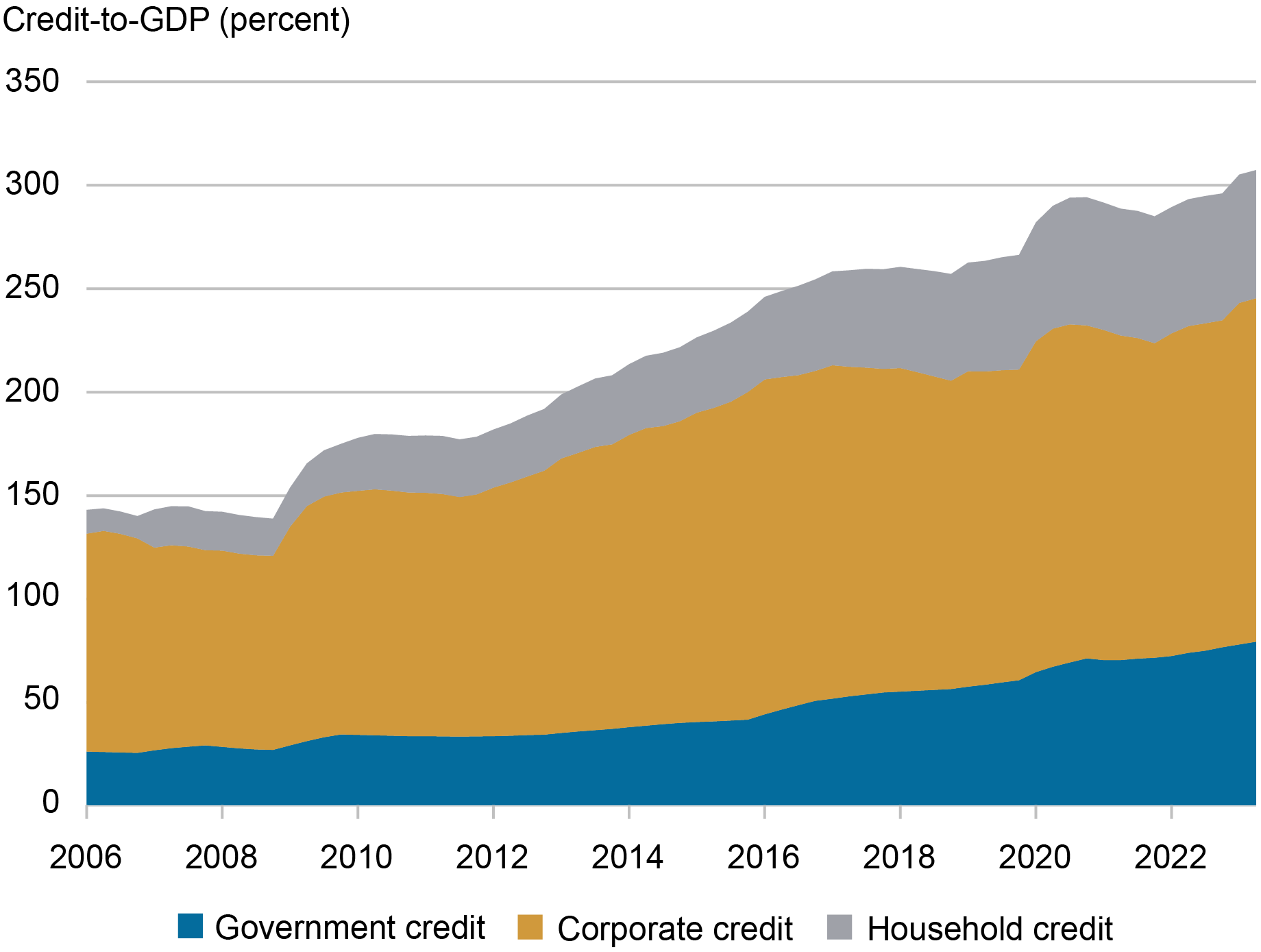 Sources: CEIC; Bank for International Settlements.
The Potential for Another Leg Down in the Property Sector
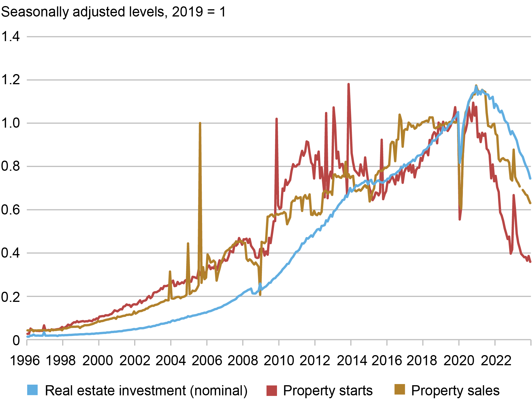
The key driver for our downside scenario would be further stress in the property sector. Since late 2020, new property starts and sales have fallen by two-thirds and one-third, respectively (chart below). Lending to developers came to a nearly complete halt through the end of 2022 before modest net lending resumed when government policy on property sector lending was eased. But total active construction projects have fallen a much smaller 13 percent since peaking in 2021, with stronger state-owned or supported developers continuing work on uncompleted projects. Construction activity could fall further if stronger developers begin to face increased financial pressure.
Further stress in the property sector would amplify ongoing fiscal tightening at the local level. In this case, unique features of China’s political and economic system would work against it. Local governments have traditionally derived a large portion of their revenues from land sales, a source that dries up in a falling price environment. In turn, these fiscal pressures would undermine local governments’ ability to support developers and other local firms, including local manufacturing champions.
Could Property Sector Activity Fall Further?
 Sources: CEIC; Authors’ calculations.
Note: Figures are calculated from official published levels.
The key role of the property sector in the Chinese economy makes troubles there a plausible trigger for an economic hard landing and financial crisis. Property-related activity accounted for roughly one-quarter of Chinese GDP before the recent slump and still represents an outsized share of activity by international standards. Property-related credit continues to account for roughly one-quarter of total debt outstanding. And property accounts for roughly two-thirds of household assets. Given this backdrop, it’s no surprise that the property slump has coincided with a severe erosion in household and business confidence.
A Downside Scenario for China and Its Implications for the U.S.
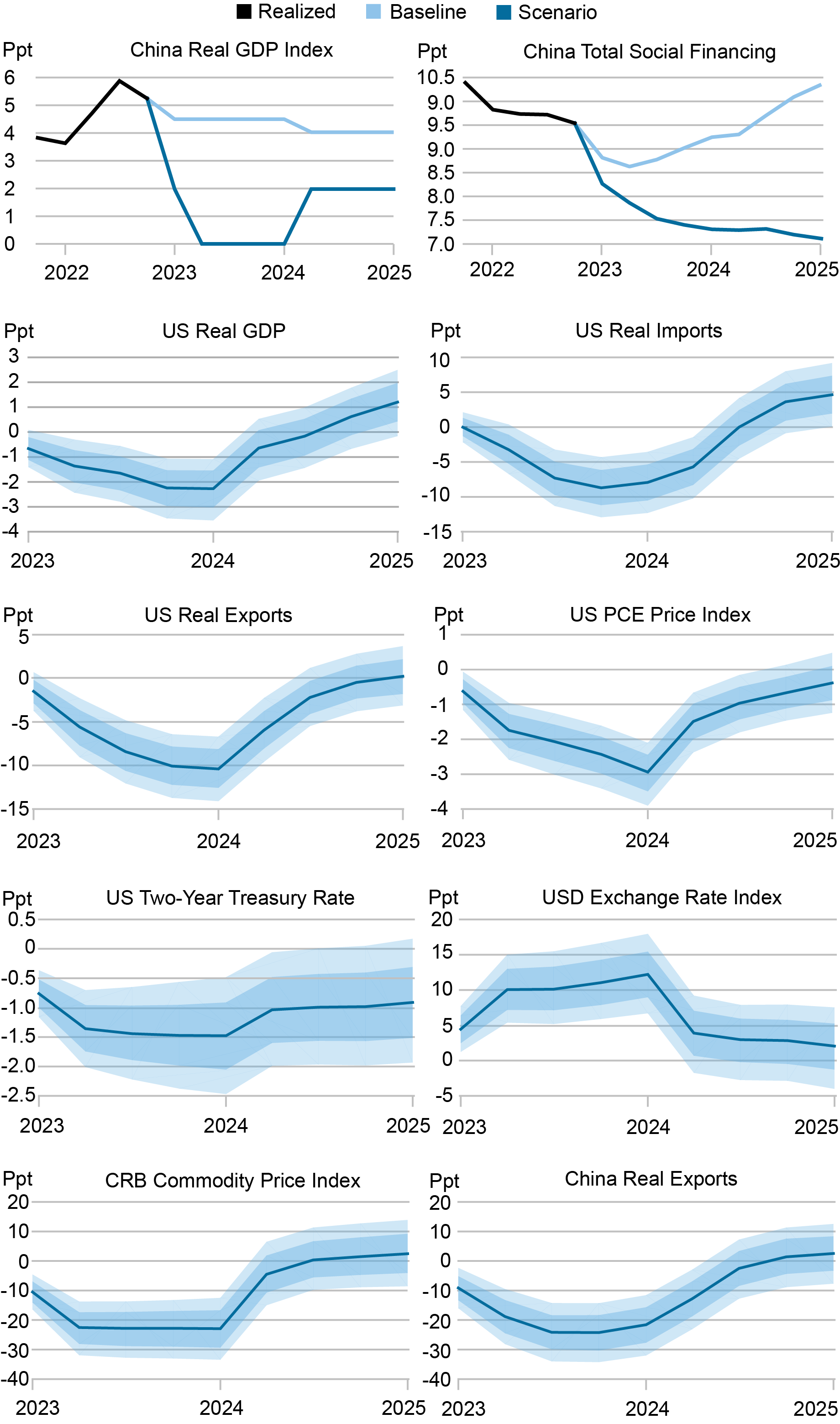
Under our property crash scenario, GDP growth in China falls to zero in 2024. This is followed by a tepid recovery to about 2 percent over the next year. This level represents dramatic underperformance relative to the International Monetary fund (IMF) baseline, which calls for growth of 4.6 percent in 2024 and 4.0 percent the following year. Credit growth (total social financing) also falls below the IMF baseline, albeit less dramatically.
To quantify the impact of this downside scenario on the U.S. economy, we rely on the Bayesian VAR model introduced in our previous post. This model is designed to capture the historical joint dynamics of the U.S. and Chinese economies. We use the estimated model relationships to construct counterfactual paths for U.S. macroeconomic aggregates while constraining Chinese output and credit growth to follow the paths in our crash scenario. As in our previous exercise, we measure scenario impacts against a baseline in which the Chinese economy evolves according to the IMF projections.
The top two panels in the chart below show the behavior of GDP and credit growth—our key conditioning variables—under the crash and baseline scenarios, reported as year-over-year percent changes. As already noted, the crash scenario involves dramatic GDP-growth underperformance relative to the baseline. The remaining panels show the implications of the crash scenario for U.S. and selected Chinese and global macro variables, measured as percentage deviations from the baseline, with the blue shading showing estimated confidence intervals.
This exercise shows that a Chinese hard landing could result in materially weaker U.S. growth and trade performance and lower U.S. inflation, with the largest impacts occurring over the first four quarters following a crash. Real GDP growth falls as much as 2 percentage points (ppt) below baseline before beginning to recover, while export volumes fall as much as 10 ppt below baseline. The PCE price index, for its part, falls some 3 ppt below baseline before crisis impacts begin to fade.
Projected Path for Key Macro Variables in a Hard Landing Scenario
 Source: Authors’ calculations based on data from the Federal Reserve Bank of St. Louis FRED database and CEIC.
The magnitude of these impacts is larger than in our earlier post premised on a manufacturing-led boom in China, consistent with the larger deviation of GDP growth from baseline. The underlying mechanisms are however the same, albeit now working in the opposite direction.
The sudden plunge in Chinese domestic demand growth leads to sharp falls in global commodity prices and Chinese exports. These impacts reflect the key role China plays in global trade and production networks. Weaker Chinese demand translates into weaker demand for China’s worldwide value chain partners, with this impact amplified by the knock-on tightening of those firms’ financing constraints. The deterioration in global trade, of course, feeds into the similar deterioration in U.S. trade volumes.
The U.S. dollar, meanwhile, sees significant appreciation, in line with its longstanding negative correlation with global commodity prices. In the context of our property crash scenario, this strength can be understood as reflecting risk-off behavior among global investors, who seek refuge in U.S. financial markets and U.S. dollar assets. The stronger dollar, in turn, contributes to a tightening in global financial conditions. In fact, the main impact of weaker Chinese demand on global financial conditions is via this indirect channel.
In short, the materialization the property crash scenario in China would tilt the balance of risks for U.S. growth and inflation to the downside. As we’ve discussed, however, the Chinese authorities appear to have adequate tools to contain new downward pressures on the country’s economy. At present, we regard the materialization of this scenario as less likely than the upside manufacturing boom scenario.
The two scenarios, of course, would carry different policy implications. A deep Chinese slowdown would contribute to lower U.S. and global inflation, likely bringing forward investor expectations for policy easing. In contrast, materially faster growth in China might add to the challenges of bringing inflation back to central bank targets, likely pushing out investor expectations for easing.

Ozge Akinci is head of International Studies in the Federal Reserve Bank of New York’s Research and Statistics Group.

Hunter L. Clark is an international policy advisor in International Studies in the Federal Reserve Bank of New York’s Research and Statistics Group.

Jeffrey B. Dawson is an international policy advisor in International Studies in the Federal Reserve Bank of New York’s Research and Statistics Group.

Matthew Higgins is an economic research advisor in International Studies in the Federal Reserve Bank of New York’s Research and Statistics Group.

Silvia Miranda-Agrippino is a research economist in International Studies in the Federal Reserve Bank of New York’s Research and Statistics Group.

Ethan Nourbash is a research analyst in the Federal Reserve Bank of New York’s Research and Statistics Group.

Ramya Nallamotu is a senior research analyst in the Federal Reserve Bank of New York’s Research and Statistics Group.
How to cite this post:
Ozge Akinci, Hunter Clark, Jeff Dawson, Matthew Higgins, Silvia Miranda-Agrippino, Ethan Nourbash, and Ramya Nallamotu, “What Happens to U.S. Activity and Inflation if China’s Property Sector Leads to a Crisis?,” Federal Reserve Bank of New York Liberty Street Economics, March 26, 2024, https://libertystreeteconomics.newyorkfed.org/2024/03/what-happens-to-u-....

Is China Running Out of Policy Space to Navigate Future Economic Challenges?

Financial Crises and the Desirability of Macroprudential Policy

Why Are China’s Households in the Doldrums?
Disclaimer
The views expressed in this post are those of the author(s) and do not necessarily reflect the position of the Federal Reserve Bank of New York or the Federal Reserve System. Any errors or omissions are the responsibility of the author(s).
The Gilded Cage: Technology, Development, and State Capitalism in China – review
In The Gilded Cage: Technology, Development, and State Capitalism in China, Ya-Wen Lei explores how China has reshaped its economy and society in recent decades, from the era of Chen Yun to the leadership of Xi Jinping. Lei’s meticulous analysis illuminates how China’s blend of marketisation and authoritarianism has engendered a unique techno-developmental capitalism, writes George Hong Jiang.
 Twenty years ago, people inside and outside China were wondering whether the country would eventually capitulate to dominant capitalist and democratic models. American politicians such as Bill Clinton were enthusiastically looking forward to the future integration of China into globalisation. When this happened, millions of ordinary people would get rich and become the middle class through fast-growing international trade and domestic labour-intensive industries. However, this judgment quickly proved ill-made. China has simultaneously emulated the US in high-tech industries but also become an unparalleled authoritarian state which polices its citizens through intellectual technology and high-tech instruments. How has it achieved this, and what are the effects of this? Lei tries to untangle these questions in her book, The Gilded Cage: Technology, Development, and State Capitalism in China.
The author was inspired by the “birdcage economy” of Chen Yun when choosing the title of the book.[…] Statist control is the cage, and private economies, like captive birds, are only allowed to fly within the cage.
The author was inspired by the “birdcage economy” of Chen Yun when choosing the title of the book (5). Building the planned economy in the early 1950s and supporting economic reforms in the 1980s, Chen Yun was one of the most important architects of economic systems in communist China. While he was a proponent of giving more space to private economies, Chen Yun staunchly believed in the efficacy of governmental regulations. Statist control is the cage, and private economies, like captive birds, are only allowed to fly within the cage. Chen Yun was particularly cautious about liberalist reforms, such as deregulation of finance and fiscal decentralisation, and distinctly opposed to privatisation. After he died in 1995, Deng Xiaoping and his disciples, including Jiang Zemin and Hu Jintao, carried out deregulation bravely until the late 2000s. But the ideal of Chen Yun’s “birdcage economy” is never abandoned by communists who fear losing control over the society.
The 2008 financial crisis started China’s big turn of macroeconomic policies. In order to stimulate the deflated economy, the government reacted fast and invested enormous capital into a few key strategic industries, including bio-manufacturing industry and aircraft and electronic manufacturing. Ling & Naughton (2016) believe that this action signalled the watershed of China’s economic orientation. The government’s budget poured into these industries, and bureaucratic units responsible for supervision and regulation turned to interventionist policies. The trend was further strengthened after Xi Jinping, who believes that the combination of the free market economy and Leninist political principles is the best blueprint for China, ascended to the presidency in 2012.
New leadership since the 2010s wants to emulate western high-end development rather than provide low-end, cheap and labour-intensive products for the West.
The ambition to develop high-tech industries runs in tandem with the unique political system of China. Economic growth has helped sustain political legitimacy of the Chinese Communist Party (CCP) since the 1980s. Since socialism was smeared by the Cultural Revolution (1966-1976) and its disastrous economic consequences, economic growth has been identified as the most important source of political legitimacy. Economic performance has become the indicator of bureaucratic promotion, which has fused China’s politics and economies together. This political organisational mechanism makes it easier for leaders to push through any desired change and it is on this that China’s turn to techno-development (Chapter Three) is precisely based. New leadership since the 2010s wants to emulate western high-end development rather than provide low-end, cheap and labour-intensive products for the West.
Still, a key question must be answered: why are Chinese bureaucrats who care primarily about social stability and political monopoly willing to replace human labour with robots, which tends to reduce employment in the short run? In Chapter Five, the author traces the process of robotisation in firms which previously rely on cheap labour, including Foxconn. While the benefits of robotisation might be obvious to entrepreneurs aspiring to reduce costs by any means, potential instability could cause trouble for communist bureaucrats. The answer lies in the possibility that technological upgrades will lead to an enlarging economy capable of digesting more workers than it kicks out. However, it results in a dilemma: if the growth rate slows down, the appetite for mechanisation and robotisation could stir social tensions.
Seeing the chance to surpass the West in the development of high-tech industries, the Chinese Communist Party (CCP) is more than willing to strengthen control over public spheres and civil society and increase investment in the sector to achieve this.
Seeing the chance to surpass the West in the development of high-tech industries, the Chinese Communist Party (CCP) is more than willing to strengthen control over public spheres and civil society and increase investment in the sector to achieve this. As the author puts it, “the Chinese state is an unwavering believer in intellectual technology and instrumental power and employs both to enhance governance and the economy” (9). It is highly possible that with the help of an authoritarian regime and its will to develop technological capability, the dismal future that Max Weber once predicted – ie, the “iron cage of bureaucracy” in which depersonalised and ossified instrumental rationality will dominate every sphere in the society – will come sooner in China than in the West.
Economic growth is mainly driven by high-tech industries that private and state-owned capital foster, both of which must be under the control of the government, with the unified aim of rejuvenating the Chinese nation.
Karl Marx argued that productive power, including technological conditions, determines relations of production. This idea is being justified in China. A mix between marketised economies and authoritarian rule, which is penetrated by high-tech instruments, facilitate the rise of techno-developmental capitalism, as the author proposes in Chapter Nine. On the one hand, large tech companies in China have hatched one of the biggest markets in the world. On the other hand, tech professionals’ increasing demand for institutional (if not political) reforms (Chapter Eight) renders bureaucrats gradually more concerned about their social influence. For instance, Jack Ma, the boss of Alibaba, attacked the state-owned financial system and instantly got punished by the authority. China is developing a new variant of capitalism: economic growth is mainly driven by high-tech industries that private and state-owned capital foster, both of which must be under the control of the government, with the unified aim of rejuvenating the Chinese nation.
Techno-developmental capitalism is not the result of contingency, but path-dependent outcome, the direct result of China’s polities.
The author includes an excellent range of relevant materials into the book, spanning academic literature and personal interviews with private entrepreneurs and IT practitioners. Lei also bravely applies the term “instrumental rationality” in relation to China’s socioeconomic reality. In so doing she identifies the Janus-faced nature of China’s technological development, whereby the society enjoys higher productivity but becomes more rigid and occluded due to the omnipotent techno-bureaucracy. Nonetheless, the book could have been improved if Lei could take China’s political-economic structure into account when explaining the motivation to develop high-tech industries. While Lei focuses on the era after the 2000s, the rise of techno-developmental capitalism is deeply rooted in the persistent logic of the CCP since the late 1970s. In other words, techno-developmental capitalism is not the result of contingency, but a path-dependent outcome, the direct result of China’s polity. In spite of this lack of fully examined historical dimensions, Lei presents a good guidebook for China’s holistic development, not just within the last two decades but also in the decades to come.
Note: This post gives the views of the author, and not the position of the LSE Review of Books blog, or of the London School of Economics and Political Science.
Image credit: B.Zhou on Shutterstock.
The European Union’s New Risk-Based Framework for Fiscal Rules – Overly Complex, Opaque and Self-Defeating
The discrepancy between technocratic rhetoric and economic facts is colossal.
Introduction and Summary
On February 10th, 2024, representatives of the European Council, the European Parliament (EP), and the European Commission (EC) reached an agreement on yet another reform of the fiscal rules.[1] The legislative package still has to be approved by both the European Council and the European Parliament by the end of April 2024. While the new rules have thus far received little attention, they will shape the fate of the European Union (EU) economy for years. After a decade of partial relaxations of its older super-restrictive rules that pushed the euro area into a prolonged recession in the years 2011-2013, and the activation of a general escape clause in the wake of multiple shocks (pandemic, energy crisis), the rules will abruptly turn restrictive again, though less so than the old ones. But if the new rules go into force, their effect on the socio-ecological transformation and the European welfare state will still be profoundly disastrous.
In announcing the agreement of the Trilogue negotiations, Vincent Van Peteghem, the finance minister of Belgium, which holds the EU presidency in the first half of 2024, claimed that the new framework “will safeguard balanced and sustainable public finances, strengthen the focus on structural reforms, and foster investments, growth and job creation throughout the EU.”[2]
This is not correct. The discrepancy between technocratic rhetoric and economic facts is just colossal. The new rules will impede, not foster growth and job creation, and they put the Euro area on track for another deadly cycle of austerity that sowed the seeds for the rise of the far-right in Europe. They admittedly build in some incentives to raise public investment, but this step implicitly comes with new pressures to restrain non-investment budgetary categories, such as social expenditures. Further, austerity programs threaten to curb economic performance, which will work against the reduction of the debt ratio which is a central objective of the new governance framework. Even though significant long-term investments in the socio-ecological transformation and in the strengthening of Europe as a business location more generally are desperately needed, the necessary investments are insufficiently protected and promoted in the agreement. In fact, the new fiscal framework will severely constrain an increase in public investment, in particular in high-debt EU countries.
Estimates of the additional public investments required to decarbonize the EU economy by 2050 vary widely.[3] The most recent study estimates the additional public investment requirement to be around 1,6% of the current EU GDP per year (Institut Rousseau 2024) which can be considered a lower bound. At 1,3% EU military spending in 2022 has been relatively stable as a percentage of GDP in the period 2013-2022 – fluctuating between 1,2 and 1,3% of GDP[4] - but this is expected to increase strongly in the upcoming years. The new rules are particularly worrisome at the back of the resistance to setting up a permanent EU investment facility – e.g. a Recovery and Resilience Fund 2.0. (RRF). A trilemma is clearly visible: An increase in public (capital) investment, fiscal consolidation, and reluctance to introduce or increase wealth tax revenues are incompatible. If the new rules are implemented the trilemma will most likely be resolved by substantially retrenching the welfare state.[5]
The methodology spelled out to assess the binding consolidation paths for countries in the new agreement is Baroque almost to a point of bizarreness and it bears a risk of procyclicality. Particularly worrisome is the use of a Debt Sustainability Analysis (DSA) to calibrate the consolidation path for each EU member state. A DSA can be considered useful to analyze fiscal risks under different scenarios with regard to growth, interest rates, or aging costs. But using this methodology – the details still have to be published - to calibrate a multiannual, binding net expenditure trajectory is an audacious undertaking. The DSA is highly judgemental, replete with self-fulfilling features, and hence is ill-suited for the operationalization of hard fiscal rules.
How Do the New Fiscal Rules Work?
Each member state is required to submit “Fiscal-Structural Plans” (FSPs) for the next four or five years to the EC. These FSPs set out strategies for sustainable public debt reduction - central to the FSPs will be the trajectory of the main operational target, the nominal growth rate of primary net expenditures – as well as strategies for inclusive growth, structural reforms, and investment. Reference is also made to the pillar of social rights, energy security, and possible defense spending as part of the FSPs. All these elements have, of course, to be compatible with the net expenditure path.
The European Commission has an essential role to play, as it examines these plans when they are submitted and subsequently monitors the annual progress. Formally, the European Council continues to decide on the basis of the Commission’s analysis to approve the plans or impose sanctions in the event of deviations.[6] Member states may also ask for an extension of the SFPs from four up to seven years which allows them to consolidate less per year and fulfil fiscal targets later. But the extension requires an increase in nationally financed public investments. The direction taken therefore depends on how the EC – and subsequently the European Council – assess the envisaged structural reforms and investments. In any case, the discretionary scope of the EC with regard to national fiscal policy strategies is considerable.
At the heart of the FSPs will be the trajectory of the main operational target, the nominal growth rate of net expenditures. The primary net expenditure path for the adjustment period will be provided by the EC and will be – after technical consultation with the member states - incorporated in the FSPs. The European Council then decides on a multi-year net expenditure path for the respective country – on the basis of a recommendation from the EC.
The definition of net expenditure is crucial for the assessment of the new fiscal rules.[7] It is defined to avoid procyclicality as it should not be affected by the operation of automatic stabilizers and other expenditure fluctuations outside government control. Further, it allows for the financing of additional expenditures with additional discretionary revenues (e.g. wealth taxes). However, public investments are not deducted from net expenditure, as the “golden rule” of public finances would have stipulated. The idea behind the golden rule is that effective public investment can both benefit future generations and, via its growth-enhancing effects, increase debt sustainability. Hence, exempting these expenditures from the calculation of expenditures may be economically justified. On a positive note, the national co-financing share within the framework of EU programs, for example, is excluded from the definition of net expenditures. Hence, national co-financing is not restricted by the expenditure rule. However, national co-financing only plays a negligible role up to now.
The net expenditure path for each country is derived in such a way that minimum adjustments have to apply so-called “safeguards” that should ensure sustainable fiscal positions at the end of the adjustment period. The latter is defined as a (structural) budget deficit ratio of no more than 1,5% and a debt ratio that is on a plausibly downward trajectory or stays at prudent levels. Hence, the net expenditure indicator is in fact the operational target, but it is endogenous to safeguards that are defined as follows:
- DSA (Debt Sustainability Analysis) safeguard: The EC conducts a DSA for each member state with the goal of deriving a reference fiscal adjustment path consistent with declining or stabilizing public debt ratio by the end of the adjustment period (see European Commission 2022 for the current EC methodology). Further, the debt ratio at the end of the adjustment period must exceed the debt ratio five years after the adjustment period with sufficiently high probability, as assessed by the Commission’s stochastic analysis. The DSA is used, so the argument goes, to preserve the country-specific nature of fiscal adjustment requirements.
- Debt sustainability safeguard: Members states with a debt level of over 90% of GDP must reduce it by an average of at least 1 percentage point each year. Members states with a debt level between 60% and 90% of GDP must reduce it by 0.5 percentage points each year.
- Deficit resilience safeguard: For countries with more than 60% of GDP public debt or more than 3% of GDP budget deficit the overall budget deficit should not be higher than 1.5% of GDP. When it is higher, the annual improvement in the structural primary balance should be 0.4% of GDP when the adjustment lasts for four years; With an extended adjustment period of seven years, the annual minimum adjustment of the structural primary balance ratio is 0.25 percentage points.
Each safeguard provides an adjustment requirement for the structural primary balance; the respective strictest safeguard is the binding constraint that is ultimately converted into the multiannual net primary expenditure path (reference path). The adjustment has to be linear to avoid backloading of fiscal consolidation; the no-backloading requirement could be considered as another important safeguard which, however, can be relaxed in particular circumstances.[8]
In general, escape clauses apply to individual member states as well as to all member states if particular circumstances outside of the control of the member state(s) have a major impact on public finances, provided it does not endanger fiscal sustainability in the medium term.
An overall assessment
On average, the consolidation requirements in the proposed framework are less stringent than those under the current fiscal rules (Darvas et al. 2023). However, with the new fiscal framework, the consolidation efforts in some countries will still be significant. Based on estimates provided by the think tank Bruegel[9] the Table below shows the annual minimum consolidation efforts for the EU-27 under the new EU fiscal framework, measured by the annual change in the structural primary balance (SPB) in percent of GDP.
Simultaneity in fiscal contraction potentially increases fiscal multipliers and bears the risk of self-defeating, i.e. contractionary fiscal consolidation: Strikingly, the six largest EU countries without Germany (Italy, France, Spain, the Netherlands, Poland, and Belgium) that together account for around half of EU GDP, have – with the exception of some smaller countries – the highest consolidation requirements, measured by the average annual change of structural primary balances in percent of GDP (see Table below). Italy, for example, has to consolidate by around 1% of GDP annually, France and Spain by around 0,8% of GDP if the shorter adjustment period is chosen. This implies possible simultaneous fiscal contractions which – via cross-border spillovers – will most likely aggravate the negative growth effects of fiscal consolidation.
The envisaged ‘counter-cyclicality’ of the net expenditure rule is at risk of becoming pro-cyclical: The single, operational binding indicator, the net primary expenditures, is defined in such a way as to avoid pro-cyclicality. However, the calibration of the net expenditure path is constrained by the strictest applicable safeguard – which is, in many of the cases, the DSA. In an economic downturn that is not considered exceptional, countries are obliged to stick to the consolidation path. This may undermine the operation of automatic stabilizers and inhibit discretionary countercyclical fiscal policy reactions to the economic downturn.
The fiscal framework is overly complex and obstructs democratic legitimacy; the controversial and opaque “structural balance” remains an important variable: The fundamental objective of reducing the complexity of the new fiscal rules was clearly missed. Although net primary expenditure growth is, at first sight, the single, binding operational fiscal target, in fact, structural budget ratios remain as imperative calculation, target, and control variables (Fiskalrat 2024). The derivation of the consolidation requirements thus becomes even more of a "black box" which impedes accountability and democratic legitimacy. Moreover, the calibration of the primary net expenditure path is based on medium-term forecasts (four or five years for the FSPs plus ten years for the DSA – thereof five years for the stochastic probability projections) and will be affected by forecasting errors. This applies, among other things, in particular to variables that are susceptible to notable revisions, such as the unobservable output gap and the interest rate, which are used to estimate the primary structural balances.

The DSA which becomes an important element in designing the fiscal trajectories of individual member states has problematic and – to some extent – self-fulfilling features. The new fiscal framework is often called “risk-based” because the EC uses a DSA as the basis for one of the safeguards to calibrate the net primary expenditure trajectory. The precise DSA methodology used for the implementation of the fiscal rules is not yet known.[10] The DSA toolkit of the EC currently in place consists of a range of projection scenarios for government debt over the next ten years: first, a baseline scenario in which compliance with the consolidation path is assumed, second, six deterministic scenarios - three deterministic stress tests (e.g. adverse ‘r-g’ differential) and three alternative fiscal policy scenarios – plus, finally, stochastic probability projections.
If this sounds implausibly complicated, it is. The methodology itself has some features that can be judged farcical at best. For example, one of the alternative fiscal policy scenarios (‘lower structural primary balances’) assumes that after a short period following the end of the adjustment period fiscal consolidation efforts stall permanently – which in some cases would result in unsustainable debt paths in the long term. To avoid this the required fiscal adjustment path then becomes more restrictive. To simplify this absurdity: The new rules implicitly assume that they will be breached later and, in anticipating this, the consolidation path is tightened. This seems to be the main reason why according to estimates based on the current EC methodology for the DSA,[11] in most of the countries that have a debt ratio that is higher than 60%, the DSA safeguard is the strictest among the safeguards.
By definition, any DSA is subjective and judgemental as it relies on assumptions and/or market expectations, in particular with regard to fiscal (e.g. fiscal costs of aging), financial (borrowing rates), and macroeconomic variables (e.g. potential output growth). Hence, the chosen methodology strongly affects the outcome. Moreover, significant forecast errors for projections for such a long period are unavoidable. If for instance potential output is projected to be too low in the DSA this will imply higher fiscal adjustment needs which, via the fiscal multiplier, will become self-fulfilling. Lower growth will then potentially bring about a result the governance framework wants to avoid: higher debt (and deficit) ratios.
Another limitation of the DSA is that cross-border spillovers are not taken into account (Heimberger 2023), which, however, might be substantial (Eller et al. 2017). The EC assumes a fiscal multiplier of 0.75, meaning that a fiscal consolidation of 1 percentage point reduces GDP growth by 0.75 percentage points in the same year compared to the baseline. In’t Veld (2013) finds that the negative growth effects of fiscal consolidation can be notably higher when countries consolidate simultaneously (see also Heimberger 2017).
While in principle a DSA can be a useful tool for analyzing the fiscal risks under different scenarios with regard to growth, interest rates, aging costs, etc., financial markets can be very sensitive to their details. their results. Given this sensitivity, the use of DSA is very delicate. Using this tool to calibrate a multiannual, binding net expenditure trajectory is a fairly bold endeavor. Why have members of the Economic and Financial Affairs Council (ECFIN)[12] and the Committee on Economic and Monetary Affairs (ECON) of the European Parliament,[13] without knowing the precise, still-to-be-published details, voted in favor of this Rube Goldberg framework is a separate research question.
The new fiscal rules allow the EC a wide scope for decision-making while neglecting the need for appropriate democratic accountability: This holds particularly for the decision on requested extensions of the multiannual FSPs which allows for lower fiscal adjustments of the member states. A member state can extend the required adjustment path from four up to seven years if it credibly assures that it intends to make growth-promoting investments, among other things, but also if it implements EC recommendations for structural reforms as part of the European Semester. Hence, the EU Council may – at the recommendation of the EC – press member states to implement particular structural reforms. This would be a dramatic shift from the usual practice where the EC can only issue recommendations that are non-binding. To give the DSA an enhanced role in the fiscal governance framework moreover strongly limits democratic legitimacy as this tool is opaque and difficult to comprehend for policymakers. Regrettably, the same holds true for the overall fiscal governance framework.
The regulation of the new fiscal framework contains numerous references to the involvement of the social partners and to the European pillar of social rights. For example, the countries should set out in their FSPs which measures they are planning to implement in order to accomplish the European pillar of social rights. But at the same time, they should also explain how they are implementing the EC's recommendations as part of the “European Semester” which is often aimed at deregulating economies. While references to social issues can be considered as "soft law", where the EC has a high degree of discretion in their interpretation, the net expenditure path needs to be implemented as "hard law" - otherwise sanctions may be imposed.
The opportunity to foster temporary (green) public investments, e.g. by excluding public investment expenditures from the safeguards and/or implementing a ‘golden rule’, was largely missed: With the new fiscal rules public investments can only be increased if discretionary revenues rise in parallel, e.g. via a wealth tax, and/or if member states undertake more fiscal consolidation in non-investment components (e.g. social expenditures). The new rules also raise questions about the Recovery and Resilience Fund (RRF) 2.0 which is supposed to become a permanent EU investment fund. The RRF currently in place expires at the end of 2026. Calls for the extension of the EU fiscal capacity were dismissed. Given the need for rising public investments and the requested rising defense expenditures a significant retrenchment of the European welfare state is the likely outcome should the new fiscal rules materialize, with vast consequences for Europe’s social and political system.
References
Darvas, Z., L. Welslau and J. Zettelmeyer. A quantitative evaluation of the European Commission’s Fiscal governance proposal. Bruegel Working Paper 16/2023. https://www.bruegel.org/sites/default/files/2023-09/WP%2016_3.pdf
Eller, M; Feldkircher, M and F. Huber. How would a fiscal shock in Germany affect other European countries? Evidence from a Bayesian GVAR model with sign restrictions. Focus on European Economic Integration 1/2017.
European Commission (2022), Debt Sustainability Monitor. Institutional Paper 199, April 2023. https://economy-finance.ec.europa.eu/publications/debt-sustainability-monitor-2022_en
Fiskalrat (2024). Neuer Fiskalrahmen der EU – neue Komplexität. Kursanalyse des Büros des Fiskalrats Austria, https://www.fiskalrat.at/publikationen/studien-des-bueros/kurzanalysen-informationen-uebersicht.html
Heimberger P. Did Fiscal Consolidation Cause the Double-Dip Recession in the Euro Area?', Review of Keynesian Economics, Vol. 5, No. 3, 2017, pp. 539-558 .
Heimberger P. (2023). Debt sustainability analysis as an anchor in EU fiscal rules. An assessment of the European Commission’s reform orientations. In depth analysis requested by the ECON committee of the European Parliament. March 2023. https://www.europarl.europa.eu/RegData/etudes/IDAN/2023/741504/IPOL_IDA(2023)741504_EN.pdf
Heimberger P and Andreas Lichtenberger, 2023. "RRF 2.0: A Permanent EU Investment Fund in the Context of the Energy Crisis, Climate Change and EU Fiscal Rules," wiiw Policy Notes 63, The Vienna Institute for International Economic Studies, wiiw. https://wiiw.ac.at/rrf-2-0-a-permanent-eu-investment-fund-in-the-context-of-the-energy-crisis-climate-change-and-eu-fiscal-rules-dlp-6425.pdf
In ’t Veld, J. (2013): Fiscal consolidations and spillovers in the Euro area periphery and core. European Economy – Economic Papers 506.
Institut Rousseau, Road to Net Zero. Bridging the Green Investment Gap. https://institut-rousseau.fr/road-2-net-zero/
Notes
[1] The legislative package consists of a regulation on the preventive arm (Regulation on the effective coordination of economic policies and multilateral budgetary surveillance – final compromise text following the trilogue agreement) as well as a directive (Directive on requirements for budgetary frameworks of the Member States - Agreement in principle with a view to consulting the EP) and a regulation on the corrective arm (Regulation on speeding up and clarifying the implementation of the excessive deficit procedure - Agreement in principle with a view to consulting the EP).
[2] https://www.consilium.europa.eu/en/press/press-releases/2024/02/10/economic-governance-review-council-and-parliament-strike-deal-on-reform-of-fiscal-rules/
[3] For an overview see Heimberger and Lichtenberger 2022.
[4] See https://ec.europa.eu/eurostat/statistics-explained/index.php?title=Government_expenditure_on_defence#Expenditure_on_.27defence.27
[5] Christian Lindner, German Finance minister, has recently provided insights into what might be awaiting us. He has urged a moratorium on social expenditures and subsidies to finance public military expenditures. This view was supported by Clemens Fuest, President of the IFO Institute. https://www.faz.net/aktuell/wirtschaft/lindner-fordert-moratorium-bei-sozialausgaben-19540142.html.
[6] An excessive deficit procedure (EDP) can be opened a) if the 3% deficit ratio threshold is breached or b) if there is a significant deviation from the specified net primary expenditure path. Deviations from the expenditure path are noted in a control account and an EDP procedure is triggered if thresholds are exceeded (0.3% of GDP in one year or cumulatively by 0.6% of GDP). In this case, however, an EDP is only opened if the public debt ratio is higher than 60% and the deficit ratio is higher than 0,5%.
If an EDP is opened, member states have to adjust their primary structural balance ratio by 0.5 percentage points. While they may initially exclude interest payments, after 2027 exclusion of interest payments is no longer possible which makes little sense.
[7] ‘Net expenditure’ means government expenditure net of interest expenditure, discretionary revenue measures, expenditure on programs of the Union fully matched by Union funds revenue, national expenditure on co-financing of programs funded by the Union, cyclical elements of unemployment benefit expenditure, and one-offs and other temporary measures.
[8] A member state may request an exemption to the no-backloading safeguard. This has to be taken into account if the respective country has projects related to the Recovery and Resilience Facility loans as well as national co-financing of EU funds in 2025 and 2026.
[9] See https://www.jvi.org/fileadmin/jvi_files/News/2024/24WR02_Feb21/2024-02-21_Greening_EU_fiscal_rules.pdf
[10] The methodology will be described in the Debt Sustainability Monitor 2023 that will be published in April 2024.
[11] See for example, https://www.jvi.org/fileadmin/jvi_files/News/2024/24WR02_Feb21/2024-02-21_Greening_EU_fiscal_rules.pdf
[12] The new fiscal rules were approved by the members of the EU Economic and Financial Affairs Council (ECFIN) by 8th December 2023.
[13] The new fiscal rules were approved by the members of the Committee on Economic and Monetary Affairs (ECON) of the European Parliament by 5th of March 2024.