Monetary policy
Is UK monetary policy driving private housing rents?
Daniel Albuquerque and Jamie Lenney

Rent prices have risen by 9% on average in England since the Bank of England’s Monetary Policy Committee (MPC) started raising interest rates in December 2021. Alongside this rise in prices has been a widening in the gap between reported supply and demand in the rental sector, with tenant demand continuing to rise in 2023 amidst falling supply (RICS survey). Is monetary policy causing the rise in rents? In this post, we provide evidence that temporary increases in interest rates are ultimately associated with a decrease in rental prices that follows an initial, but relatively short lived, increase in rental prices and tenant demand. These results also hold across regions in England.
Rising rents and monetary policy
The recent rise in rents will be of significant concern to the 19% of households in the UK that are private renters, for whom housing costs already take up 33% of their income on average. Despite the fact that rising interest rates have been implemented to reduce overall price inflation, monetary policy has been cited as a possible cause of rising rental prices principally through two channels. First, the resulting increase in mortgage costs has consequences for both supply and demand in the rental market: it can discourage new buy-to-let landlords, and keep future homeowners as tenants for longer. Second, housing is an investable asset, and returns on other assets are rising due to the increase in interest rates. Thus, even non-mortgagor landlords are likely to increase rents in response to rising interest rates to match the expected return on other assets.
However, empirical evidence is mixed – in the US, for example, economists at the San Francisco Fed find that rents immediately decline in response to rising interest rates, while other work has documented increases in rental prices without a subsequent decline.
So is there any evidence that monetary policy is pushing up rental prices in the UK?
Estimating the causal effect of monetary policy on the rental market
In order to answer this question we use a local projections framework with 12 lags of the variable of interest as controls. We rely on monetary policy surprises identified in the 30-minute windows around MPC announcements to estimate the effect of monetary policy on rental prices, as described in more detail by Cesa-Bianchi et al (2020). We use unexpected changes (surprises) to identify the effect of monetary policy because most interest rate changes are made in response to current and future economic conditions. Simply using all interest rate changes would mix up the effect of interest rates on rental prices with the effects of other shocks that interest rates are trying to counteract.
For rental prices, we use data from ONS’s Index of Private Housing Rental Prices from 2005 to 2019, for England. We focus on England because data for the whole of the UK is available from 2015 only. We choose to end our data sample in 2019: we exclude the Covid pandemic period, because the relationship between monetary policy and rental prices may have changed during this time; and we have insufficient lags of data to make it worthwhile including data post-pandemic.
Chart 1 shows the estimated response of housing rents to a 1 percentage point rise in interest rates. The response for England as a whole is the dark blue line with the 1 standard deviation confidence interval shaded in blue. We also plot the point estimates for each English region in grey. The point estimates indicate rental prices rise by around 1% over the 12 months following a rise in interest rates. This result is replicated in most regions in England with the exception of the East Midlands, where the central estimate shows no rise in rents. Chart 1 also shows that after around 12 months this rise begins to dissipate, and by month 22 the point estimate is below zero in all regions.
Chart 1: The response of private rental prices to a 1 percentage point rise in interest rates

Note: The blue shaded region is the 1 standard deviation confidence interval for England.
Does the response of rental prices make sense?
As noted above, since housing is an asset, when real interest rates rise the real return on housing should ultimately also rise in line with other available returns. This real return can be achieved by either rising rents or falling house prices, or some combination of the two. Using the same local projections framework as in Chart 1, Panel A in Chart 2 shows that rental yields (rent divided by house price) do indeed rise in response to rising interest rates. Panel B decomposes this response in rental yields for England between movements in rental prices and movement in house prices (the latter is calculated as a residual).
Chart 2: Response of rental yields to a 1 percentage point rise in interest rates, and its decomposition between yield and house prices movements

Note: The blue shaded region is the 1 standard deviation confidence interval for England.
As Chart 2B shows, rental prices increase initially, in line with the increase in rental yields. However, our estimates suggest that most of the adjustment is coming from falling house prices, even though that adjustment is sluggish and takes almost a full year to materialise. As house prices are slow to adjust, this puts pressure on rents to rise at first in order for landlords to make adequate returns relative to their outside option ie selling and investing in other assets like government bonds. At the same time, we find that housing transactions fall in the year following the interest rate rise (Chart 4A uses the local projections frameworks from before on UK Land registry data for housing transactions). This slowdown in housing transactions can help explain a reduction in the supply of rental housing if selling landlords take their property off the rental market but struggle to find prospective buy-to-let landlords who, discouraged by rising mortgage rates, need house prices to fall further to make adequate returns.
Using survey data on the residential market provided by RICS and household panel data from Understanding Society we can also analyse the effect of monetary policy on tenant demand. Panel A in Chart 3 uses a similar framework as used in Chart 1 to plot the response of the reported net balances of changes in tenant demand in the rental market in the RICS survey. It shows that a rise in interest rates is initially associated with a rise in tenant demand that then dissipates after around a year. In Panel B, using individual panel data, we show that the estimated probability of home ownership falls for younger cohorts in the 12 months following a rise in interest rates. This helps to partially explain the rise in tenant demand through a delay in the transition from renting to owning.
Chart 3: Tenant demand after a 1 percentage point rise in interest rates

Note: The blue shaded regions are 1 standard deviation confidence intervals.
So initially rising interest rates could well cause pricing pressures in the rental market. However, over time house prices fall due to tighter monetary policy and enable new landlords to come in and offer lower rents. At the same time, households are likely to become increasingly unwilling to accept and afford rent increases as the effect of monetary policy on their real income builds. This gradual transmission of monetary policy to broader economic activity and incomes is illustrated in Panel B of Chart 4, which uses a similar framework to that of Cesa-Bianchi et al (2020) to show an estimate for the effect of a 1 percentage point rise in interest rates on GDP. Panel B shows GDP falling gradually with the peak impact occurring after around 12 months and persisting beyond that.
Chart 4: The gradual response of housing transactions and economic activity to a 1 percentage point rise in interest rates

Note: The blue shaded region is the the 1 standard deviation confidence interval.
Rental prices in context today
The causal effect of monetary policy in any given cycle is always difficult to disentangle from other broader shocks. This is especially true today with the UK in the midst of a broader inflationary shock, and still recovering from the longer-run economic effects of Covid that upended housing markets and migration flows. It is also worth noting that there have been changes in regulations affecting the rental market. These shocks are both directly and indirectly the underlying drivers of rising rents. Chart 5 plots the rise in private rents since December 2021 alongside the rise in average earnings and the level of CPI services. Both have tracked and indeed outgrown the rise in private rental prices, meaning that the relative cost of renting on average has not risen since interest rates started to increase. Compared to our results this is somewhat surprising, as our analysis would suggest rents could be growing faster than wages or other services now. However, other shocks to the UK’s labour market or cost pressures in specific sectors make it difficult to be definitive in this statement. Overall, through the lens of Chart 5, the pressures in the rental market seem to be consistent with the broader supply constraints in the economy.
Chart 5: Rental prices relative to incomes and other prices

Note: Prices are in levels and normalised to 100 at December 2021. Earnings are average weekly labour earnings.
Summing up
This post suggests that interest rate rises decrease rental prices in the long run, but that they may initially put pressure on the rental market. In our analysis, a temporary rise in interest rates leads to temporary increases in rental yields, as happens for returns on other assets in the economy. Tenant demand rises at first and landlord supply may be dampened by rising mortgage costs and slow adjustment of house prices. However, over time, our results indicate that the housing market should adjust, causing rental prices to decline.
Daniel Albuquerque and Jamie Lenney work in the Bank’s Monetary Policy and Outlook Division.
If you want to get in touch, please email us at bankunderground@bankofengland.co.uk or leave a comment below.
Comments will only appear once approved by a moderator, and are only published where a full name is supplied. Bank Underground is a blog for Bank of England staff to share views that challenge – or support – prevailing policy orthodoxies. The views expressed here are those of the authors, and are not necessarily those of the Bank of England, or its policy committees.
Dropping Like a Stone: ON RRP Take‑up in the Second Half of 2023

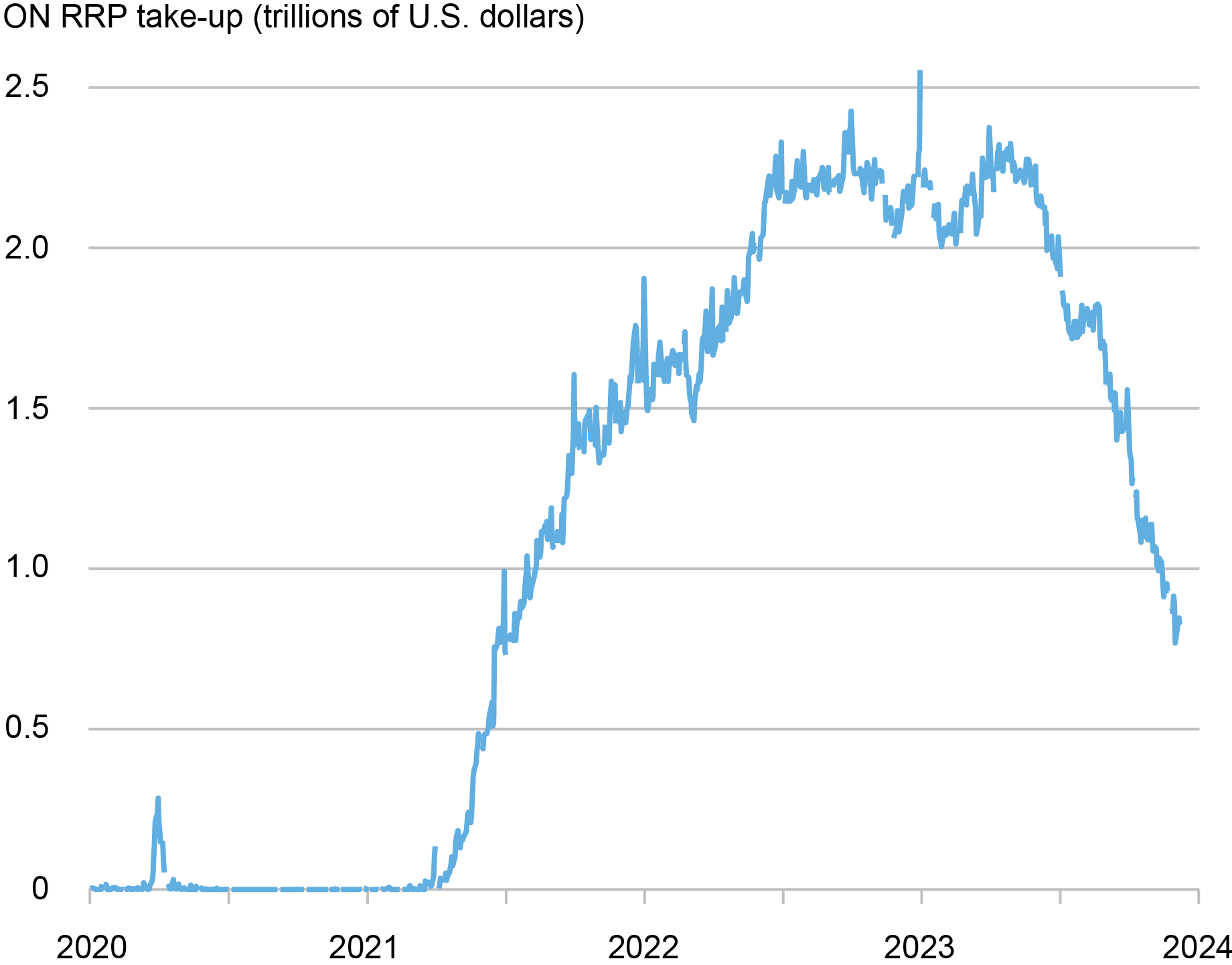
Take-up at the Overnight Reverse Repo Facility (ON RRP) has halved over the past six months, declining by more than $1 trillion since June 2023. This steady decrease follows a rapid increase from close to zero in early 2021 to $2.2 trillion in December 2022, and a period of relatively stable balances during the first half of 2023. In this post, we interpret the recent drop in ON RRP take-up through the lens of the channels that we identify in our recent Staff Report as driving its initial increase.
ON RRP Take-up Has Been Decreasing since June 2023…
 Source: Federal Reserve of St. Louis. FRED database.
Banks’ Balance-Sheet Costs
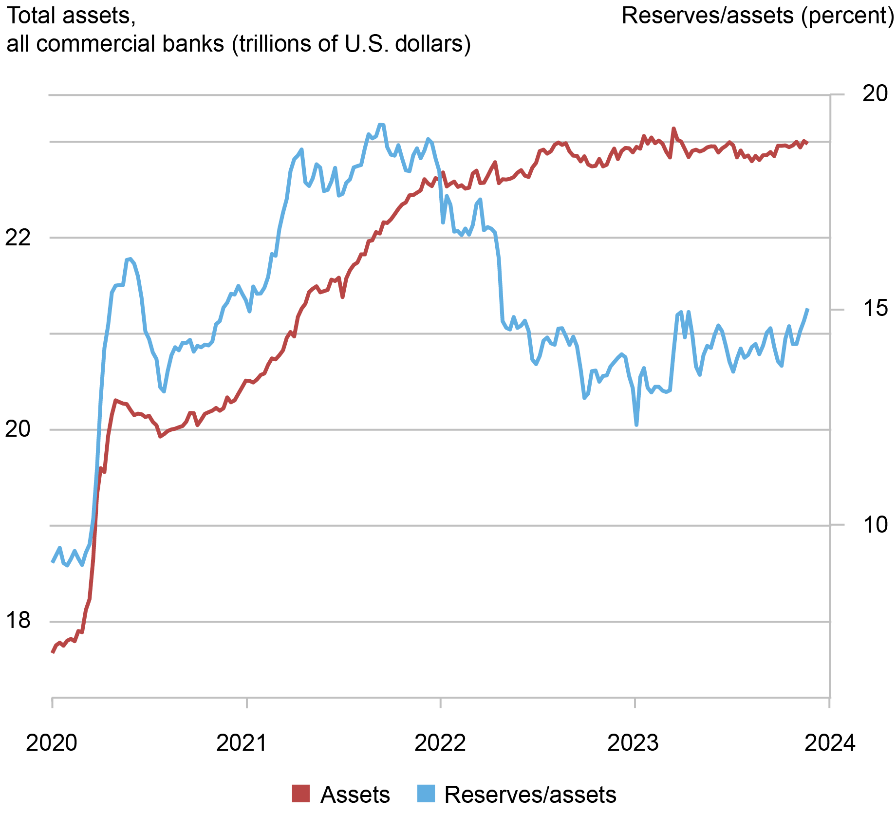
As the Federal Reserve expanded its balance sheet in response to the COVID-19 pandemic, it increased the supply of reserves to the banking system and, as a result, banks’ balance sheets also grew. Reserves increased from $1.6 trillion—or 9 percent of banks assets—in January 2020 to $3.2 trillion—or 16 percent of bank assets—over the following three months, reaching a historical maximum of 19 percent of banks’ assets in September 2021. As the chart below shows, bank assets also grew from $18 trillion in January of 2020 to $20 trillion in April 2020, and continued to increase to $23 trillion in May 2023.
As banks’ balance sheets expand, regulatory ratios—such as the supplementary leverage ratio (SLR)—are likely to become tighter for some institutions. Banks react to increased balance-sheet costs by pushing some of their deposits toward the money market fund (MMF) industry—for instance, by lowering the rate paid on bank deposits—and reducing their demand for short-term debt. As we explain in our paper, both effects are likely to have boosted ON RRP take-up during March 2021 – May 2023, as most MMFs are eligible to invest in the ON RRP and do so especially when alternative investment options, such as banks’ wholesale short-term debt—including repos by dealers affiliated with a bank holding company—dwindle.
Likely, these effects have subsided relative to 2022. Indeed, since June 2023, bank assets have hovered around $23 trillion, slightly below their March 2023 peak. Moreover, reserves have been around 14 percent of bank assets since June 2023, below the average of 16 percent observed between March 2020 and May 2023. Since the SLR treats all assets in the same way regardless of their riskiness, large banks’ balance-sheet expansions are particularly costly if they are used to finance safe assets with low returns. Therefore, though bank assets have remained relatively stable, the recent decline in the ratio of reserves to bank assets has likely reduced banks’ overall balance-sheet costs.
…while Bank Assets and Reserves Relative to Bank Assets Have Remained Roughly Constant.
 Source: Federal Reserve Bank of St. Louis. FRED database.
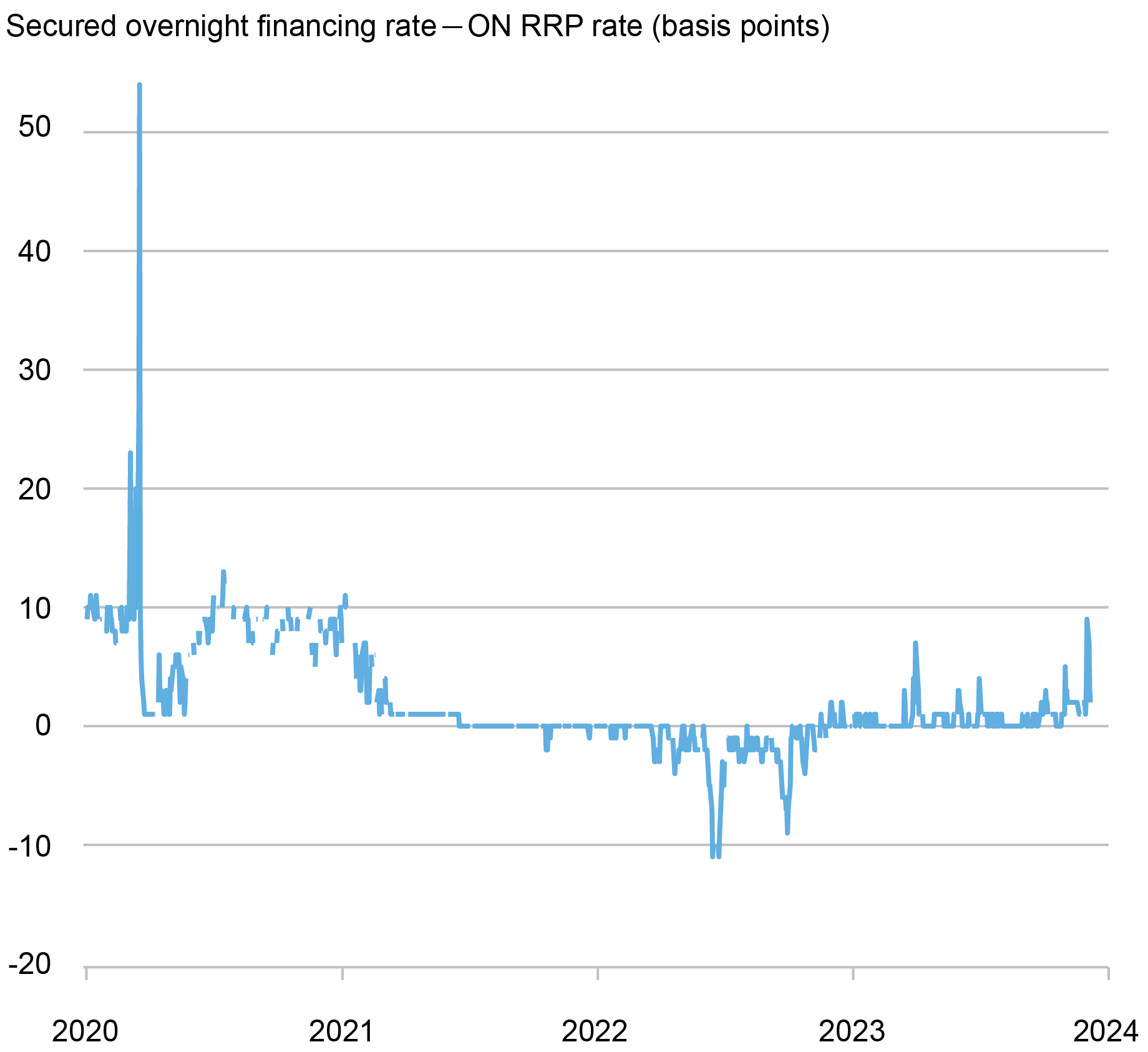
Consistent with a decrease in banks’ balance-sheet costs (and an increase in the supply of bank debt), the interest rates at which banks and broker dealers borrow via overnight Treasury-backed repos have increased since the fourth quarter of 2022 and are now a few basis points above the ON RRP rate (see chart below). This positive rate differential pushes MMFs away from investing at the ON RRP facility and into private repos.
The SOFR-ON RRP Spread Has Been Positive…
 Source: Federal Reserve of St. Louis, FRED database.
Monetary Policy
Monetary policy can affect ON RRP take-up by MMFs in two ways. First, the interest-rate pass-through of MMF shares is higher than that of bank deposits; as a result, the size of the MMF industry comoves with the monetary policy cycle as investors switch from bank deposits to MMF shares when the policy rate increases. Though the assets of the MMF industry are at an all-time high, the pace of the increase has somewhat decreased recently, consistent with a slower pace of monetary policy tightening; moreover, the share of MMF assets managed by government funds—the ones most likely to invest in the ON RRP—has decreased since June 2022 by 7 percentage points.
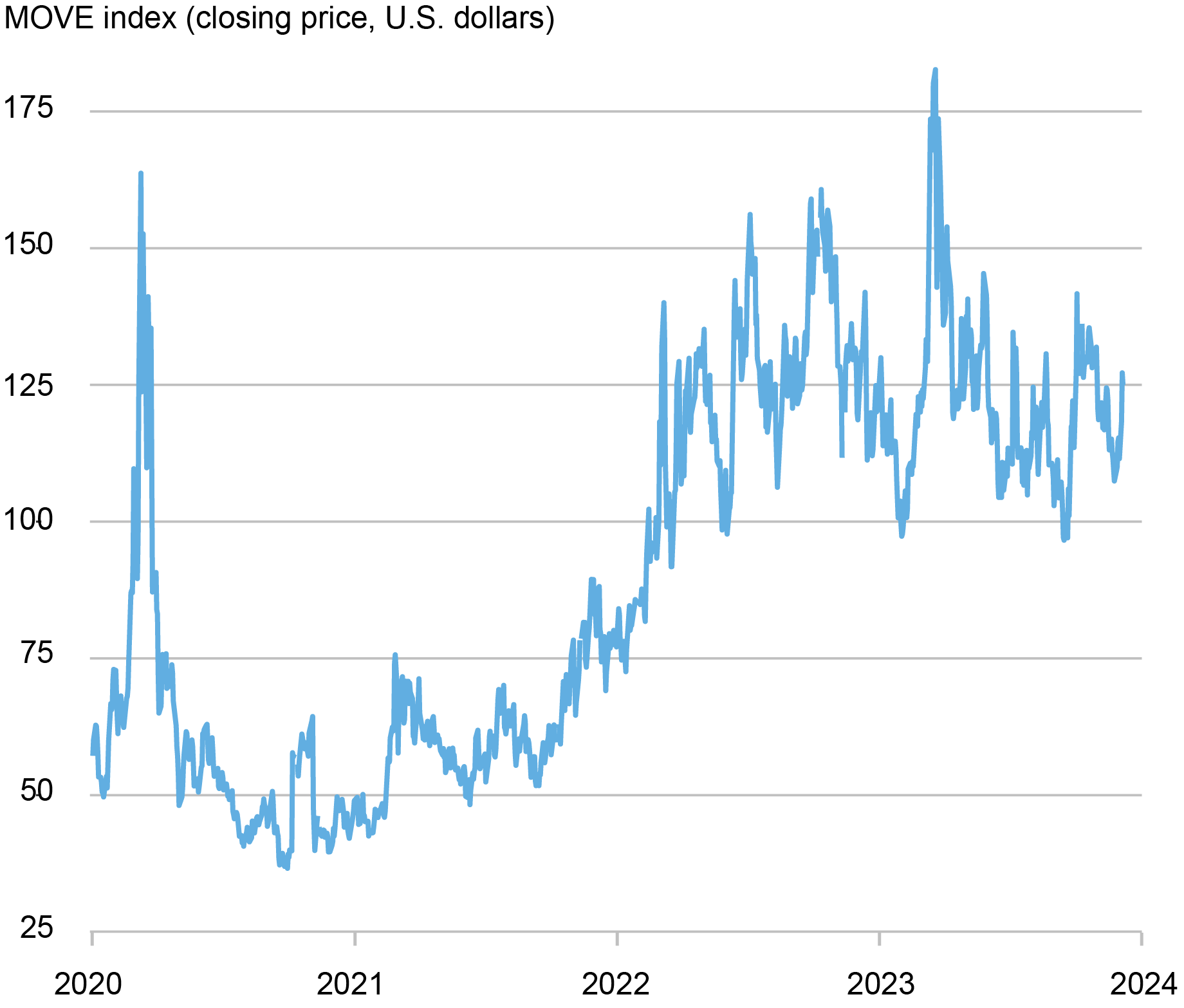
Second, monetary policy can affect MMFs’ take-up at the ON RRP also through its effect on interest-rate uncertainty. Higher uncertainty leads MMFs to rebalance their portfolios toward investments with shorter duration; the ON RRP is one such investment as it is overnight. Indeed, interest rate uncertainty—as measured by the MOVE index—had increased substantially during the latest tightening cycle, raising from 57.3 in May 2021 to 136 in May 2023. Recently, however, the increase has been partially reversed. Indeed, the average level of the MOVE was 125.6 in the first half of 2023 but declined to 117.3 in the second half of the year.
…while Interest-Rate Uncertainty Has Been Decreasing.
 Source: Yahoo! Finance.
The Supply of T-bills
A third driver of ON RRP take-up is the supply of T-bills. The Federal Government has expanded the supply of T-bills dramatically in 2023: T-bills outstanding increased from $3.7 trillion at the end of 2022 to $5.3 trillion at the end of September 2023, with a $1.3 trillion increase since June. As the supply of T-bills grows, the investment options of MMFs—and especially of government funds, which represent 83 percent of the industry and can only invest in short-term government debt and repos backed by government debt—expand and, as a result, their investment in the ON RRP dwindles. In our staff report, we estimate that a $100 billion increase in the amount of T-bill issuance reduces the proportion of ON RRP investment in a government-MMF portfolio by 2.3 percentage points, relative to that in a prime-MMF portfolio; since average monthly T-bill issuance went from $1.12 trillion in the period from 2022:Q1-2023:Q1 to $1.53 trillion in 2023:Q2-2023:Q3, this effect on portfolio rebalancing amounts to an additional decrease in ON RRP investment of roughly $350 billion.
Summing It Up
The increase in ON RRP take-up between 2021 and May 2023 was driven by a series of factors: a rise in banks’ balance-sheet costs due to the expansion of the supply of reserves in response to the COVID-19 pandemic, the rapid hikes in policy rates aimed at fighting inflation and the resulting increase in interest-rate uncertainty, and the decrease in the T-bill supply of 2021-22 resulting from the normalization of public debt after the COVID-19 crisis.
These factors have reversed: the Federal Reserve restarted running off its balance sheet after the temporary expansion during the banking turmoil of March 2023; the growth of the banking system waned while the ratio of reserves to asset decreased; the pace of interest-rate hikes slowed down; and the T-bill supply increased again. If these dynamics persist in the months ahead, ON RRP take-up may continue to decrease. Such a steady decline would be consistent with that observed in early 2018, when investment at the ON RRP gradually disappeared as the Federal Reserve continued to normalize the size of its balance sheet and reserves in the banking system became less abundant.

Gara Afonso is the head of Banking Studies in the Federal Reserve Bank of New York’s Research and Statistics Group.

Marco Cipriani is the head of Money and Payments Studies in the Federal Reserve Bank of New York’s Research and Statistics Group.

Gabriele La Spada is a financial research economist in Money and Payments Studies in the Federal Reserve Bank of New York’s Research and Statistics Group.
How to cite this post:
Gara Afonso, Marco Cipriani, and Gabriele La Spada, “Dropping Like a Stone: ON RRP Take‑up in the Second Half of 2023,” Federal Reserve Bank of New York Liberty Street Economics, December 19, 2023, https://libertystreeteconomics.newyorkfed.org/2023/12/dropping-like-a-st....

Banks’ Balance-Sheet Costs, Monetary Policy, and the ON RRP
Monetary Policy Transmission and the Size of the Money Market Fund Industry: An Update

The Transmission of Monetary Policy and the Sophistication of Money Market Fund Investors
Disclaimer
The views expressed in this post are those of the author(s) and do not necessarily reflect the position of the Federal Reserve Bank of New York or the Federal Reserve System. Any errors or omissions are the responsibility of the author(s).
Hetzel Withholds Credit from Hawtrey for his Monetary Explanation of the Great Depression
In my previous post, I explained how the real-bills doctrine originally espoused by Adam Smith was later misunderstood and misapplied as a policy guide for central banking, not, as Smith understood it, as a guide for individual fractional-reserve banks. In his recent book on the history of the Federal Reserve, Robert Hetzel recounts how the Federal Reserve was founded, and to a large extent guided in its early years, by believers in the real-bills doctrine. On top of their misunderstanding of what the real-bills doctrine really meant, they also misunderstood the transformation of the international monetary system from the classical gold standard that had been in effect as an international system from the early 1870s to the outbreak of World War I. Before World War I, no central bank, even the Bank of England, dominant central bank at the time, could determine the international price level shared by all countries on the gold standard. But by the early 1920s, the Federal Reserve System, after huge wartime and postwar gold inflows, held almost half of the world’s gold reserves. Its gold holdings empowered the Fed to control the value of gold, and thereby the price level, not only for itself but for all the other countries rejoining the restored gold standard during the 1920s.
All of this was understood by Hawtrey in 1919 when he first warned that restoring the gold standard after the war could cause catastrophic deflation unless the countries restoring the gold standard agreed to restrain their demands for gold. The cooperation, while informal and imperfect, did moderate the increased demand for gold as over 30 countries rejoined the gold standard in the 1920s until the cooperation broke down in 1928.
Unlike most other Monetarists, especially Milton Friedman and his followers, whose explanatory focus was almost entirely on the US quantity of money rather than on the international monetary conditions resulting from the fraught attempt to restore the international gold standard, Hetzel acknowledges Hawtrey’s contributions and his understanding of the confluence of forces that led to a downturn in the summer of 1929 followed by a stock-market crash in October.
Recounting events during the 1920s and the early stages of the Great Depression, Hetzel mentions or quotes Hawtrey a number of times, for example, crediting (p. 100) both Hawtrey and Gustav Cassel, for “predicting that a return to the gold standard as it existed prior to World War I would destabilize Europe through deflation.” Discussing the Fed’s exaggerated concerns about the inflationary consequences of stock-market spectulation, Hetzel (p. 136) quotes Hawtrey’s remark that the Fed’s dear-money policy, aiming to curb stock-market speculation “stopped speculation by stopping prosperity.” Hetzel (p. 142) also quotes Hawtrey approvingly about the importance of keeping value of money stable and the futility of urging monetary authorities to stabilize the value of money if they believe themselves incapable of doing so. Later (p. 156), Hetzel, calling Hawtrey a lone voice (thereby ignoring Cassel), quotes Hawtrey’s scathing criticism of the monetary authorities for their slow response to the sudden onset of rapid deflation in late 1929 and early 1930, including his remark: “Deflation may become so intense that it is difficult to induce traders to borrow on any terms, and that in that event the only remedy is the purchase of securities by the central bank with a view to directly increase the supply of money.”
In Chapter 9 (entitled “The Great Contraction” in a nod to the corresponding chapter in A Monetary History of the United States by Friedman and Schwartz), Hetzel understandably focuses on Federal Reserve policy. Friedman insisted that the Great Contraction started as a normal business-cycle downturn caused by Fed tightening to quell stock-market speculation that was needlessly exacerbated by the Fed’s failure to stop a collapse of the US money stock precipitated by a series of bank failures in 1930, and was then transmitted to the rest of the world through the fixed-exchange-rate regime of the restored gold standard. Unlike Friedman Hetzel acknowledges the essential role of the gold standard in not only propagating, but in causing, the Great Depression.
But Hetzel leaves the seriously mistaken impression that the international causes and dimensions of the Great Depression (as opposed to the US-centered account advanced by Friedman) was neither known nor understood until the recent research undertaken by such economists as Barry Eichengreen, Peter Temin, Douglas Irwin, Clark Johnson, and Scott Sumner, decades after publication of the Monetary History. What Hetzel leaves unsaid is that the recent work he cites largely rediscoveed the contemporaneous work of Hawtrey and Cassel. While recent research provides further, and perhaps more sophisticated, quantitative confirmation of the Hawtrey-Cassel monetary explanation of the Great Depression, it adds little, if anything, to their broad and deep analytical and historical account of the downward deflationary spiral from 1929 to 1933 and its causes.
In section 9.11 (with the heading “Why Did Learning Prove Impossible?”) Hetzel (p. 187) actually quotes a lengthy passage from Hawtrey (1932, pp. 204-05) describing the widely held view that the stock-market crash and subsequent downturn were the result of a bursting speculative bubble that had been encouraged and sustained by easy-money policies of the Fed and the loose lending practices of the banking system. It was of course a view that Hawtrey rejected, but was quoted by Hetzel to show that contemporary opinion during the Great Depression viewed easy monetary policy as both the cause of the crash and Great Depression, and as powerless to prevent or reverse the downward spiral that followed the bust.
Although Hetzel is familiar enough with Hawtrey’s writings to know that he believed that the Great Depression had been caused by misguided monetary stringency, Hetzel is perplexed by the long failure to recognize that the Great Depression was caused by mistaken monetary policy. Hetzel (p. 189) quotes Friedman’s solution to the puzzle:
It was believed [in the Depression] . . . that monetary policy had been tried and had been found wanting. In part that view reflected the natural tendency for the monetary authorities to blame other forces for the terrible economic events that were occurring. The people who run monetary policy are human beings, even as you and I, and a common human characteristic is that if anything bad happens it is somebody else’s fault.
Friedman, The Counter-revolution in Monetary Theory. London: Institute for Economic Affairs, p. 12.
To which Hetzel, as if totally unaware of Hawtrey and Cassel, adds: “Nevertheless, no one even outside the Fed [my emphasis] mounted a sustained, effective attack on monetary policy as uniformly contractionary in the Depression.”
Apparently further searching for a solution, Hetzel in Chapter twelve (“Contemporary Critics in the Depression”), provides a general overview of contemporary opinion about the causes of the Depression, focusing on 14 economists—all Americans, except for Joseph Schumpeter (arriving at Harvard in 1932), Gottfried Haberler (arriving at Harvard in 1936), Hawtrey and Cassel. Although acknowledging the difficulty of applying the quantity theory to a gold-standard monetary regime, especially when international in scope, Hetzel classifies them either as proponents or opponents of the quantity theory. Remarkably, Hetzel includes Hawtrey among those quantity theorists who “lacked a theory attributing money to the behavior of the Fed rather than to the commercial banking system” and who “lacked a monetary explanation of the Depression highlighting the role of the Fed as opposed to the maladjustment of relative prices.” Only one economist, Laughlin Currie, did not, in Hetzel’s view, lack those two theories.
Hetzel then briefly describes the views of each of the 14 economists: first opponents and then proponents of the quantity theory. He begins his summary of Hawtrey’s views with a favorable assessment of Hawtrey’s repeated warnings as early as 1919 that, unless the gold standard were restored in a way that did not substantially increase the demand for gold, a severe deflation would result.
Despite having already included Hawtrey among those lacking “a theory attributing money to the behavior of the Fed rather than to the commercial banking system,” Hetzel (p. 281-82) credits Hawtrey with having “almost alone among his contemporaries advanced the idea that central banks can create money,” quoting from Hawtrey’s The Art of Central Banking.
Now the central bank has the power of creating money. If it chooses to buy assets of any kind, it assumes corresponding liabilities and its liabilities, whether notes or deposits, are money. . . . When they [central banks] buy, they create money, and place it in the hands of the sellers. There must ultimately be a limit to the amount of money that the sellers will hold idle, and it follows that by this process the vicious cycle of deflation can always be broken, however great the stagnation of business and the reluctance of borrowers may be.
Hawtrey, The Art of Central Banking: London: Frank Cass, 1932 [1962], p. 172
Having already quoted Hawtrey’s explicit assertion that central banks can create money, Hetzel struggles to justify classifying Hawtrey among those denying that central banks can do so, by quoting later statements that, according to Hetzel, show that Hawtrey doubted that central banks could cause a recovery from depression, and “accepted the . . . view that central banks had tried to stimulate the economy, and . . . no longer mentioned the idea of central banks creating money.”
Efforts have been made over and over again to induce that expansion of demand which is the essential condition of a revival of activity. In the United States, particularly, cheap money, open-market purchases, mounting cash reserves, public works, budget deficits . . . in fact the whole apparatus of inflation has been applied, and inflation has not supervened.
Hawtrey, “The Credit Deadlock” in A. D. Gayer, ed., The Lessons of Monetary Experience, New York: Farrar & Rhinehart, p. 141.
Hetzel here confuses the two distinct and different deficiencies supposedly shared by quantity theorists other than Laughlin Currie: “[lack] of a theory attributing money to the . . . Fed rather than to the commercial banking system” and “[lack] of a monetary explanation of the Depression highlighting the role of the Fed as opposed to the maladjustment of relative prices.” Explicitly mentioning open-market purchases, Hawtrey obviously did not withdraw the attribution of money to the behavior of the Fed. It’s true that he questioned whether the increase in the money stock resulting from open-market purchases had been effective, but that would relate only to Hetzel’s second criterion–lack of a monetary explanation of the Depression highlighting the role of the Fed as opposed to the maladjustment of relative prices—not the first.
But even the relevance of the second criterion to Hawtrey is dubious, because Hawtrey explained both the monetary origins of the Depression and the ineffectiveness of the monetary response to the downturn, namely the monetary response having been delayed until the onset of a credit deadlock. The possibility of a credit deadlock doesn’t negate the underlying monetary theory of the Depression; it only suggests an explanation of why the delayed monetary expansion didn’t trigger a recovery as strong as a prompt expansion would have.
Turning to Hawtrey’s discussion of the brief, but powerful, revival that began almost immediately after FDR suspended the gold standard and raised the dollar gold price (i.e., direct monetary stimulus) upon taking office, Hetzel (Id.) misrepresents Hawtrey as saying that the problem was pessimism not contractionary monetary policy; Hawtrey actually attributed the weakening of the recovery to “an all-round increase of costs” following enactment of the National Industrial Recovery Act, that dissipated “expectations of profit on which the movement had been built.” In modern terminology it would be described as a negative supply-side shock.
In a further misrepresentation, Hetzel writes (p. 282), “despite the isolated reference above to ‘creating money,’ Hawtrey understood the central bank as operating through its influence on financial intermediation, with the corollary that in depression a lack of demand for funds would limit the ability of the central bank to stimulate the economy.” Insofar as that reference was isolated, the isolation was due to Hetzel’s selectivity, not Hawtrey’s understanding of the capacity of a central bank. Hawtrey undoubtedly wrote more extensively about the intermediation channel of monetary policy than about open-market purchases, inasmuch as it was through the intermediation channel that, historically, monetary policy had operated. But as early as 1925, Hawtrey wrote in his paper “Public Expenditure and the Demand for Labour”:
It is conceivable that . . . a low bank rate by itself might be found to be an insufficient restorative. But the effect of a low bank rate can be reinforced by purchase of securities on the part of the central bank in the open market.
Although Hawtrey was pessimistic that a low bank rate could counter a credit deadlock, he never denied the efficacy of open-market purchases. Hetzel cites the first (1931) edition of Hawtrey’s Trade Depression and the Way Out, to support his contention that “Hawtrey (1931, 24) believed that in the Depression ‘cheap money’ failed to revive the economy.” In the cited passage, Hawtrey observed that between 1844 and 1924 Bank rate had never fallen below 2% while in 1930 the New York Fed discount rate fell to 2.5% in June 1930, to 2% in December and to 1.5% in May 1931.
Apparently, Hetzel neglected to read the passage (pp. 30-31) (though he later quotes a passage on p. 32) in the next chapter (entitled “Deadlock in the Credit Market”), or he would not have cited the passage on p. 24 to show that Hawtrey denied that monetary policy could counter the Depression.
A moderate trade depression can be cured by cheap money. The cure will be prompter if a low Bank rate is reinforced by purchases of securities in the open market by the Central Bank. But so long as the depression is moderate, low rates will of themselves suffice to stimulate borrowing.
On the other hand, if the depression is very severe, enterprise will be killed. It is possible that no rate of interest, however low, will tempt dealers to buy goods. Even lending money without interest would not help if the borrower anticipated a loss on every conceivable use . . . of the money. In that case the purchase of securities by the Central Bank, which is otherwise no more than a useful reinforcement of the low Bank rate, hastening the progress of revival, becomes an essential condition of the revival beginning at all. By buying securities the Central Bank creates money [my emphasis], which appears in the form of deposits credited to the banks whose customers have sold the securities. The banks can thus be flooded with idle money, and given . . . powerful inducement to find additional borrowers.
Something like this situation occurred in the years 1894-96. The trade reaction which began after 1891 was disastrously aggravated by the American crisis of 1893. Enterprise seemed . . . absolutely dead. Bank rate was reduced to 2% in February 1894, and remained continuously at that rate for 2.5 years.
The Bank of England received unprecedented quantities of gold, and yet added to its holdings of Government securities. Its deposits rose to a substantially higher total than was ever reached either before or after, till the outbreak of war in 1914. Nevertheless, revival was slow. The fall of prices was not stopped till 1896. But by that time the unemployment percentage, which had exceeded 10% in the winter of 1893, had fallen to 3.3%.
Hawtrey, Trade Depression and the Way Out. London: Longmans, Green and Company, 1931.
This passage was likely written in mid-1931, the first edition having been published in September 1931. In the second edition published two years later, Hawtrey elaborated on the conditions in 1931 discussed in the first edition. Describing the context of the monetary policy of the Bank of England in 1930, Hawtrey wrote:
For some time the gold situation had been a source of anxiety in London. The inflow of “distress gold” was only a stop-gap defence against the apparently limitless demands of France and the United States. When it failed, and the country lost £20,000,000 of gold in three months, the Bank resorted to restrictive measures.
Bank rate was not raised, but the Government securities in the Banking Department were reduced from £52,000,000 in the middle of January 1931 to £28,000,000 at the end of March. That was the lowest figure since August 1928. The 3% bank rate became “effective,” the market rate on 3-months bills rising above 2.5%. Here was a restrictive open market policy, designed to curtail the amount of idle money in the banking system.
Between May 1930 and January 1931, the drain of gold to France and the United States had not caused any active measures of credit restriction. Even in that period credit relaxation had been less consistent and whole-hearted than it might have been. In the years 1894-96 the 2% bank rate was almost continuously ineffective, the market rate in 1895 averaging less than 1%. In 1930 the market rate never fell below 2%.
So, notwithstanding Hetzel’s suggestion to contrary, Hawtrey clearly did not believe that the failure of easy-money policy to promote a recovery in 1930-31 showed that monetary policy is necessarily ineffective in a deep depression; it showed that the open-market purchases of central banks had been too timid. Hawtrey made this point explicitly in the second edition (1933, p. 141) of Trade Depression and the Way Out:
When . . . expanding currency and expanding bank deposits do not bring revival, it is sometimes contended that it is no use creating additional credit, because it will not circulate, but will merely be added to the idle balances. And without doubt it ought not to be taken for granted that every addition to the volume of bank balances will necessarily and automatically be accompanied by a proportional addition to demand.
But people do not have an unlimited desire to hold idle balances. Because they already hold more than usual, it does not follow that they are willing to hold more still. And if in the first instance a credit expansion seems to do no more than swell balances without increasing demand, further expansion is bound ultimately to reach a point at which demand responds.
Trying to bolster his argument that Hawtrey conceded the inability of monetary policy to promote recovery from the Depression, Hetzel quotes from Hawtrey’s writings in 1937 and 1938. In his 1937 paper on “The Credit Deadlock,” Hawtrey considered the Fisher equation breaking down the nominal rate of interest into a real rate of interest (corresponding to the expected real rate of return on capital) and expected inflation. Hawtrey explored the theoretical possibility that agents’ expectations could become so pessimistic that the expected rate of deflation would exceed the expected rate of return on capital, so that holding money became more profitable than any capital investment; no investments would be forthcoming in such an economy, which would then descend into the downward deflationary spiral that Hawtrey called a credit deadlock.
In those circumstances, monetary policy couldn’t break the credit deadlock unless the pessimistic expectations preventing capital investments from being made were dispelled. In his gloss on the Fisher equation, a foundational proposition of monetary theory, Hawtrey didn’t deny that a central bank could increase the quantity of money via open-market operations; he questioned whether increasing the quantity of money could sufficiently increase spending and output to restore full employment if pessimistic expectations were not dispelled. Hawtrey’s argument was purely theoretical, but he believed it at least possible that the weak recovery from the Great Depression in the 1930s, even after abandonment of the gold standard and the widespread shift to easy money, had been dampened by entrepreneurial pessimism.
Hetzel also quotes two passages from Hawtrey’s 1938 volume A Century of Bank Rate to show that Hawtrey believed easy money was incapable of inducing increased investment spending and expanded output by business once pessimism and credit deadlock took hold. But those passages refer only to the inefficacy of reductions in bank rate, not of open-market purchases.
Hetzel (p. 283-84) then turns to a broad summary criticism of Hawtrey’s view of the Great Depression.
With no conception of the price system as the organizing principle behind the behavior of the economy, economists invented disequilibrium theories in which the psychology of businessmen and investors (herd behavior) powered cyclical fluctuations. The concept of the central bank causing recessions by interfering with the price system lay only in the future. Initially, Hawtrey found encouraging the Fed’s experiment in the 1920s with open market operations and economic stabilization. By the time Hawtrey wrote in 1938, it appeared evident that the experiment had failed.
Hetzel again mischaracterizes Hawtrey who certainly did not lack a conception of the price system as the organizing principle behind the behavior of the economy, and, unless Hetzel is prepared to repudiate the Fisher equation and the critical role it assigns to expectations of future prices as an explanation of macroeconomic fluctuations, it is hard to understand how the pejorative references psychology and herd behavior have any relevance to Hawtrey. And Hetzel’s suggestion that Hawtrey did not hold central banks responsible for recessions after Hetzel had earlier (p. 136) quoted Hawtrey’s statement that dear money had stopped speculation by stopping prosperity seems puzzling indeed.
Offering faint praise to Hawtrey, Hetzel calls him “especially interesting because of his deep and sophisticated knowledge of central banking,” whose “failure to understand the Great Depression as caused by an unremittingly contractionary monetary policy [is also] especially interesting.” Unfortunately, the only failure of understanding I can find in that sentence is Hetzel’s.
Hetzel concludes his summary of Hawtrey’s contribution to the understanding of the Great Depression with the observation that correction of the misperception that, in the Great Depression, a policy of easy money by the Fed had failed lay in the distant monetarist future. That dismissive observation about Hawtrey’s contribution is a misperception whose corretion I hope does not lie in the distant future.
Global R*
Ambrogio Cesa-Bianchi, Richard Harrison and Rana Sajedi

Recent increases in interest rates around the world, following a multi-decade decline, have intensified the debate on their long-run prospects. Are previous trends reversing or will rates revert to low values as current shocks subside? Answering this question requires assessing the underlying forces driving secular interest-rate trends. In a recent paper, we study the long-run drivers of the global trend interest rate – ‘Global R*’ – in the 70 years up to the pandemic. Global R* fell by more than three percentage points from its peak in the mid-1970s, driven by falling productivity growth and increased longevity. Our results suggest that without a reversal in these trends, or new forces emerging to offset them, long-run Global R* is likely to remain low.
Within a standard macroeconomic framework, secular movements in real interest rates are determined by the factors that drive the supply and demand for capital. Over the long run, when capital can move freely across countries, there exists a single interest rate that clears the global capital market. This global trend real interest rate, Global R*, acts as an anchor for domestic interest rates in open economies, so that estimates of Global R* are important inputs to longer-term structural analysis, including the design of policy frameworks. So studying the factors that drive global wealth and capital accumulation is crucial for understanding interest-rate trends around the world.
Our focus on Global R* differs from many other studies, which use closed-economy semi-structural models to estimate a higher-frequency concept of the equilibrium real interest rate: the real interest rate that stabilises output at potential and inflation at target (see, for example, Holston et al (2017)). Our approach instead aims to identify the role of longer-term global trends. We deliberately abstract from shocks that determine equilibrium real interest rates over shorter horizons in individual economies and therefore cause these shorter-term equilibrium real rates to deviate from Global R*. The distinction between equilibrium interest rates over different horizons is discussed in more detail by Bailey et al (2022) and Obstfeld (2023).
Methodology and data
We develop a structural model to study the secular drivers of interest rates. Our framework is a standard neo-classical model with overlapping generations of households. It parsimoniously captures the effects of slow-moving trends in five key drivers: productivity growth, population growth, longevity, government debt, and the relative price of capital. We treat the world as a single large (closed) economy, and each period in the model corresponds to five years.
To guide our model simulations, we construct a panel data set for these variables for 31 high-income countries with an open capital account from 1950 to 2019. This group of countries can be regarded as a good approximation to a single fully integrated closed economy. The dynamic path of each driver is estimated by extracting the low-frequency common component across countries, to capture its long-run global trend. Conditional on these observed global trends for the five drivers, which are treated as exogenous, the model generates a simulated path for Global R*.
Studies of this kind typically assume ‘perfect foresight’, meaning that agents fully anticipate the entire paths of the drivers from the start of the simulation. Since our simulations span several decades of substantial structural change, this assumption is implausible, and at odds with widespread evidence of persistent errors in forecasting low-frequency changes in the drivers (see Keilman (2001), and Edge et al (2007)). So, instead, we use a novel recursive simulation methodology that captures slow-moving beliefs about long-term trends: beliefs about the future evolution of the drivers are only partially updated each period.
To calibrate the model and to set the initial level of the interest rate at the start of the simulations, we construct an empirical estimate of Global R*, using data for the same group of countries. This empirical estimate comes from a vector autoregression (VAR) model with common trends, closely following the approach of Del Negro et al (2019), to model the joint dynamics of short-term interest rates, long-term interest rates, and inflation, using annual data from 1900 to 2019.
The evolution of Global R*
Chart 1 shows our model simulation of Global R* alongside the VAR estimate. We plot the model simulation as five-year lines, to emphasise that the model determines the interest rate for successive five-year periods, though the interest rate is shown as an annualised percentage rate.
Chart 1: Evolution of Global R* estimates

Source: Cesa-Bianchi et al (2023).
The VAR estimate of Global R* was relatively stable at around 2.25% in the first part of the sample, between 1900 and 1930. After falling to 1.25% around time of the Second World War, the VAR estimate rose again between 1950 and 1980, reaching a peak of around 2.5%. Since the 1980s, the VAR estimate of Global R* has been on a downward path, reaching 0% in recent years.
We initialise our model simulation using the VAR estimate so that, by construction, the model simulation and VAR estimates are very close in the first five-year model period (1951–55). Thereafter the simulated path rises more quickly than the VAR estimate, and peaks slightly earlier. The peak real rate of around 2.5% for 1971–75 is broadly in line with the VAR estimate at that time, lying slightly above the 68% posterior interval. Beyond the peak, the model simulation of Global R* falls more quickly than the VAR estimate reaching -0.75% by the end of the sample. Despite these differences in the level, the simulated change in Global R* from the early 1980s onward, a period that has attracted considerable interest in the literature, is almost identical to the change in our empirical estimate over the same period.
The suggestion that the global trend real interest rate could be negative may seem striking, as it would appear to be possible to finance investment projects with negative returns. However, the marginal product of capital exceeds the safe rate of return because of the mark-up charged by imperfectly competitive producers. So the marginal product of capital in our simulations is positive, even when the safe rate of return is negative.
Decomposing the drivers of Global R*
As we said at the start, an important question that our methodology is designed to answer is ‘what have been the drivers of the decline in Global R*?’. Chart 2 presents a decomposition of the change in Global R* from our model simulations. Each bar shows the contribution of an individual driver, computed by constructing a simulation in which only that driver changes over the sample (with all other drivers held fixed at their initial values).
Chart 2: Decomposition of the drivers of Global R*

Source: Cesa-Bianchi et al (2023).
The estimated decline in Global R* from its peak has been primarily driven by changes in longevity and productivity growth. Increased longevity, due to falling mortality rates in particular for over-65s, induced a greater accumulation of wealth to finance longer periods of retirement. These higher desired wealth holdings have in turn reduced Global R*. Slower trend productivity growth has also reduced Global R*, since lower expected returns on investment have reduced the demand for capital.
Higher population growth in the early part of our sample – the ‘baby boom’ – pushes up slightly on Global R*, with the effects particularly noticeable in the 1990s and 2000s. Thereafter the effect wanes but not sufficiently to push down on R* in our simulation. In line with other studies, the relative price of capital has only a modest effect on the equilibrium real interest rate. Finally, at a global level, trend movements in government debt are not sufficient to have a material impact on R* in our model.
Several other potential drivers of trend real interest rates have been investigated in previous work, but are not incorporated in our model because of the difficulty in building a reliable panel of data for the countries and time period that we study. To the extent that mark-ups, risk and inequality have been increasing over time, we would expect these factors to exert further downward pressure on Global R*. Rising retirement ages and greater provision of health and social insurance could in principle work in the opposite direction. Finally, physical impacts from climate change and the (global) transition to net zero may also affect R* through a variety of channels working potentially in different directions. More work is needed to understand these various channels, and quantify their relative importance and net effect on R*.
The outlook for Global R*
Our simulations imply that increased longevity and slowing productivity growth have resulted in a large fall in Global R*. As noted earlier, forecasting global trends is notoriously difficult. Some of these drivers could reverse, and new forces could emerge to offset them. Nevertheless, the global rise in longevity is not expected to unwind, and so its effect on Global R* is expected to persist.
Ambrogio Cesa-Bianchi works in the Bank’s International Directorate, Richard Harrison works in the Bank’s Monetary Analysis Directorate and Rana Sajedi works in the Bank’s Research Hub.
If you want to get in touch, please email us at bankunderground@bankofengland.co.uk or leave a comment below.
Comments will only appear once approved by a moderator, and are only published where a full name is supplied. Bank Underground is a blog for Bank of England staff to share views that challenge – or support – prevailing policy orthodoxies. The views expressed here are those of the authors, and are not necessarily those of the Bank of England, or its policy committees.
Why lower house prices could lead to higher mortgage rates
Fergus Cumming and Danny Walker

Bank Rate has risen by more than 5 percentage points in the UK over the past couple of years. This has led to much higher mortgage rates for many people. In this post we analyse another potential source of pressure on mortgagors: the potential for falls in house prices to push borrowers into higher – and therefore more expensive – loan to value (LTV) bands. In a scenario where house prices fall by 10% and high LTV spreads rise by 100 basis points, we estimate that an additional 350,000 mortgagors could be pushed above an LTV of 75%, which could increase their annual repayments by an extra £2,000 on average. This could have a material impact on the economy.
There is significant public and media attention on how the Bank of England’s interest rate decisions affect mortgagors. The interest rates set by central banks are of course a key determinant of the rates people pay on their mortgages. Banks tend to price mortgages off interest rate swaps, which reflect the market’s expectations of future policy rates. The relevant swap rates for the 80% of UK mortgages that have fixed interest rates are typically the two and five-year rates. While Bank Rate has risen by more than 5 percentage points since December 2021, the two-year swap rate has risen by 4.6 percentage points and two-year mortgage rates have risen by around 4.5 percentage points (Chart 1). But Bank Rate is not the only determinant of mortgage rates.
Chart 1: Mortgage rates have increased sharply in the UK – they tend to be priced off swap rates, which are linked to Bank Rate

Note: The chart shows quoted rates for two-year mortgages at different LTV ratio bands. It compares them to Bank Rate (the Bank of England policy rate) and the two-year swap rate, both of which are considered risk-free rates.
Source: Bank of England.
Mortgages with lower deposits – higher LTV ratios – have higher interest rates, but the spread is currently very low
Loosely speaking, a mortgage interest rate is made up of the risk-free rate – typically the relevant swap rate – and some compensation for risk, known as the spread. LTV ratios are the key determinant of spreads. For example, someone with a deposit of at least 25% of the value of the house at the point the mortgage is issued qualifies for a 75% LTV mortgage, which comes with a lower interest rate than if they only had a deposit worth 10% of the value. Mortgages with higher deposits, and therefore lower LTVs, are generally safer for banks because higher deposits means borrowers can withstand larger house price falls before falling into negative equity. Higher LTV mortgages tend to have higher interest rates for that reason.
Throughout the 2010s it was common for the spread between 90% and 75% LTV mortgage rates to be between 1 and 2 percentage points (Chart 1). As of August 2023, that spread was less than 0.4 percentage points. In fact, spreads have been very narrow since 2021 and the last time spreads were at today’s levels was probably in 2008, which is before the official data began. Given that high LTV mortgages look relatively cheap compared with recent history, we construct an illustrative scenario where the 90% LTV spread returns to close to its post-2010 average – something we regard as plausible.
We analyse an illustrative scenario where mortgage spreads rise by 100 basis points and house prices fall by 10% from their peak
Our aim is not to forecast what will happen in the mortgage market, but simply to examine a set of conditions that are within the realms of possibility. We use data on the universe of UK owner-occupier mortgages in the Product Sales Database. The most detailed information is recorded when mortgages are originated for the first time and upon remortgage. We build a snapshot of the mortgage market by modelling how much principal people have paid down since origination and how house prices have evolved in their region. We focus on mortgages originated since 2020 Q4 because they are most likely to have high LTV ratios, given the borrowers have not had much time to pay down principal and have had less time to benefit from significant house price increases.
In our scenario analysis, the 90% LTV mortgage rate increases by 100 basis points (Chart 2) and house prices fall by 10% (Chart 3). As a comparison, in the 2007 to 2009 financial crisis, the 90% LTV spread – measured versus 60% LTV mortgages – reached over 250 basis points and house prices fell by almost 20% from peak to trough.
Chart 2: In our scenario analysis, the interest rates on mortgages with LTV ratios of above 75% increase by 100 basis points, taking them closer to historical spreads

Note: The chart shows quoted rates for two-year mortgages at different LTV bands, expressed as a spread versus the 0%–60% LTV rate. We analyse an indicative scenario where the spread on 75%–90%, 90%–100% and 100%+ LTV mortgages rises by 100 basis points.
Source: Bank of England.
We recalculate LTVs following the 10% fall in house prices in the scenario and assume all mortgagors eventually have to refinance at the new higher rate for their LTV band. In the real world, mortgagors reaching the end of their fixed term will face a recalculation of their LTV based on a revaluation of their house, which is typically calculated using private sector indices. As it happens, those indices have already fallen by a few per cent more than the official price index shown on Chart 3. We do not model mortgage choice in the scenario: for simplicity we assume that mortgagors take out a two-year fixed-rate mortgage.
Chart 3: In our scenario analysis, UK average house prices fall by 10%, taking them back to around their 2021 level

Note: The chart shows the UK house price index expressed as a percentage change since the start of 2010. We analyse an indicative scenario where the index falls by 10%.
Sources: Bank of England and Office for National Statistics.
The scenario pushes an additional 350,000 mortgagors above 75% LTV, increasing their annual repayments by £2,000 on average
At origination, around 40% of recent mortgages had deposits that were too small to be eligible for a 0%–60% or 60%–75% LTV mortgage. When we take account of principal repayments and house price growth since origination, that suggests around a quarter of recent mortgages – just under 800,000 – are above that 75% LTV threshold now.
We find that the house price fall in our scenario pushes an additional 350,000 mortgagors above the 75% LTV threshold, taking the total back to around 40% of recent mortgagors (Chart 4), or 1.1 million. It also pushes around 3% into negative equity. The assumed 100 basis point increase in mortgage spreads in the scenario leads to an average increase in annual repayments for these mortgagors of just over £2,000 by the time they refinance, over and above the impact from the increase in swap-rates. That is clearly a material impact for the people affected, but is it material for the economy?
Chart 4: The scenario leads to a rise in LTV ratios for recent mortgagors, which comes with higher interest rates

Note: The chart shows all UK owner-occupier mortgages in the Product Sales Database originated since 2020 Q4, split by LTV ratio. We update the loan amount outstanding by modelling the scheduled flow of principal repayments for each loan. We update the house price based on an assumption that house prices have evolved in line with the average price in their region (eg London, South East of England etc). The scenario reduces prices uniformly by 10%. We assume for simplicity that there are no 80% LTV products. The numbers should be interpreted as indicative rather than a precise read on the stock of UK mortgages.
Sources: Bank of England and Financial Conduct Authority Product Sales Database.
The macro impact of this scenario could be material, given that it affects those mortgagors that are most financially constrained
At first glance, the impact of this scenario looks relatively modest in comparison to the increase in Bank Rate that has already occurred. The 100 basis point increase in mortgage spreads in our scenario is less than a quarter of the size of the rise in swap rates that has already occurred. It also only affects 40% of recent mortgagors, and just over 10% of all mortgagors. Focusing on recent mortgagors, our analysis suggests that their aggregate additional repayment burden (£2.4 billion) amounts to around 20% of the total repayment increase caused by the rise in Bank rate on its own (£11 billion).
But it is also true that the mortgagors impacted by this scenario are some of the most financially constrained households, and some of the most important for policymakers to consider. Well-established theoretical research has emphasised the role of heterogeneity in macroeconomics and empirical research has previously explored the importance of the most levered mortgagors in the transmission of monetary policy. To the extent that the scenario affects households most likely to substantially change their spending patterns, it is plausible that this amplification channel is not trivial. Indeed, for the most levered mortgagors, the scenario eventually increases repayments by 40% over-and-above the rise in mortgage rates already baked in.
Implications
Policymakers across the globe are well versed in the importance of the housing and mortgage markets, particularly for monetary policy transmission. The financial crisis is still in the rear-view mirror and much has been learned from it. But this post highlights an interesting channel of monetary policy which, while it will be captured implicitly in some models, is often less discussed outside policy circles. The scenario analysis reminds us that there can be more to monetary policy tightening than risk-free rates. Many people expect the tightening that has already occurred to lead to a significant fall in house prices, and it is plausible that mortgage spreads will return to historical levels. Although there is uncertainty, this has the potential to lead to a material impact on economic activity over and above the impact of risk-free rates.
Fergus Cumming is Deputy Chief Economist at the Foreign, Commonwealth and Development Office. He used to work on monetary policy and financial stability at the Bank. Danny Walker works in the Bank’s Deputy Governor’s office.
If you want to get in touch, please email us at bankunderground@bankofengland.co.uk or leave a comment below.
Comments will only appear once approved by a moderator, and are only published where a full name is supplied. Bank Underground is a blog for Bank of England staff to share views that challenge – or support – prevailing policy orthodoxies. The views expressed here are those of the authors, and are not necessarily those of the Bank of England, or its policy committees.
The New York Fed DSGE Model Perspective on the Lagged Effect of Monetary Policy

This post uses the New York Fed DSGE model to ask the question: What would have happened to interest rates, output, and inflation had the Federal Reserve been following an average inflation targeting (AIT)-type reaction function since 2021:Q2, when inflation began to rise—as opposed to keeping the federal funds rate at the zero lower bound (ZLB) until March 2022, and then raising it aggressively thereafter? We show that actual policy was more accommodative in 2021 than implied by the AIT reaction function and then more contractionary in 2022 and beyond. On net, the lagged effect of monetary policy on the level of GDP, when measured relative to the counterfactual, has been positive throughout the forecast horizon, due to the initial boost associated with keeping the fed funds rate near zero in 2021.
A Counterfactual: What If the Fed Had Stuck to the AIT Rule?
The AIT reaction function assumed throughout this exercise is in line with the 2020 monetary policy framework review. The parameters of the AIT rule—specifically its response to inflation and output “misses,” and its inertia (the coefficient on lagged interest rates)—were calibrated as of 2020:Q3 in order to match the expected duration of the zero lower bound (ZLB) given the economic conditions in the middle of the COVID pandemic (see here for more details).
Our purpose here is to use our DSGE model to simulate how the economy would have performed if the monetary policy rate had not deviated from the AIT reaction function starting in 2021:Q2. The exercise can be described as follows: What would have happened to the economy had the FOMC followed the reaction function that rationalized the September 2020 pledge to keep rates at the ZLB for an extended period given expectations at that time, and therefore deviated from the ZLB pledge—in accordance with the AIT rule—when inflation strayed away from this expected path starting in 2021:Q2? The results of this counterfactual experiment need to be taken with a grain of salt, of course, as they are only as good as the model that produces them.
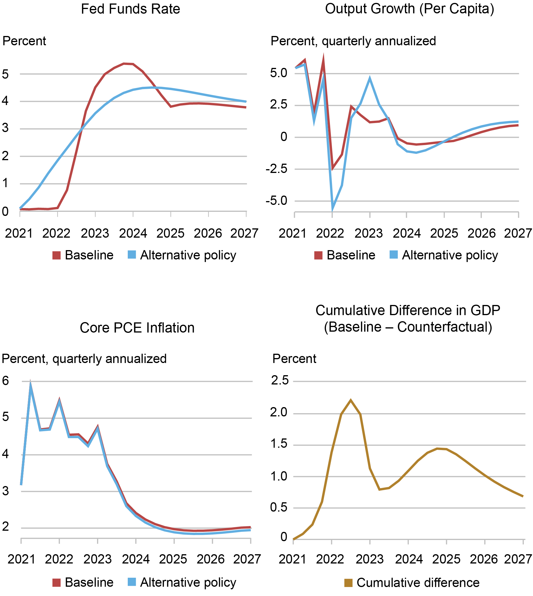
The upper left panel in the chart below shows the actual path of the fed funds rate (FFR) and the current baseline forecast after 2023:Q2 (red) versus the counterfactual path had the FOMC followed the AIT rule starting in 2021:Q2 (blue). The counterfactual path for all the variables is constructed by subjecting the counterfactual economy to the same shocks that, according to the model, have hit the actual economy, with the only difference between the two economies being the monetary policy pursued by the FOMC. So, for instance, the cost-push shocks that are the main cause for the burst in inflation (bottom left panel) in 2021 in the model (see this post) also have an impact on inflation in the counterfactual economy. Similarly, under the baseline path, we see growth rebounding in the second half of 2022 and 2023—a rebound that was due to strong demand (see this post), in line with the BVAR analysis in our accompanying post. These very shocks affect the path in the counterfactual economy as well.
Counterfactual with AIT Reaction Function Starting in 2021:Q2
Source: Authors’ calculations.
Had the FOMC followed the AIT reaction function starting in 2021:Q2, rates would have risen immediately. The counterfactual FFR path then falls below the actual FFR path in the middle of last year, remains lower than the baseline path through mid-2024, and then eventually converges from above to the actual forecasted path for interest rates. Had the FOMC pursued this policy, per capita output growth (quarterly annualized, upper right panel) would have been lower in 2022 and higher in 2023. The lower output growth in 2022 is the result of tightening in 2021, while the stronger growth this year originates from the less aggressive pace of tightening in 2022 and 2023.
The bottom right panel shows that deviations from the AIT rule have been expansionary on net. The panel shows the gap in output levels that developed starting in 2021:Q2 between the baseline and the alternative path. The counterfactual level of output is below the actual level and the gap between the two rises to a peak of about 2 percent in mid-2022, followed by a narrowing in 2023 caused by the more aggressive pace of tightening under actual policy in that year. The gap then briefly widens again in 2024-25 as actual policy eases faster than the AIT rule. On net, the lagged effect of monetary policy on economic activity, when measured relative to a counterfactual where policy follows the AIT rule, has been positive throughout the forecast horizon, due to the initial boost associated with keeping the FFR at near zero in 2021.
The lower left panel shows that inflation rates do not differ significantly between the two policy rules. This is in part because the model has a weak connection between output and inflation because of its flat Phillips curve. In part this is because in the New York Fed DSGE forecasts we have been assuming that agents in the model have been only partially aware of the change in the policy framework from inflation targeting to AIT, with a weight that increases over time. In all alternative simulations so far, we have continued to maintain this assumption: when adopting an alternative policy, the central bank was not affecting the way “unaware” agents form expectations, implying that the weakening of the economy shown in the lower right panel is not internalized by firms when setting prices.
Focusing on the Hiking Period
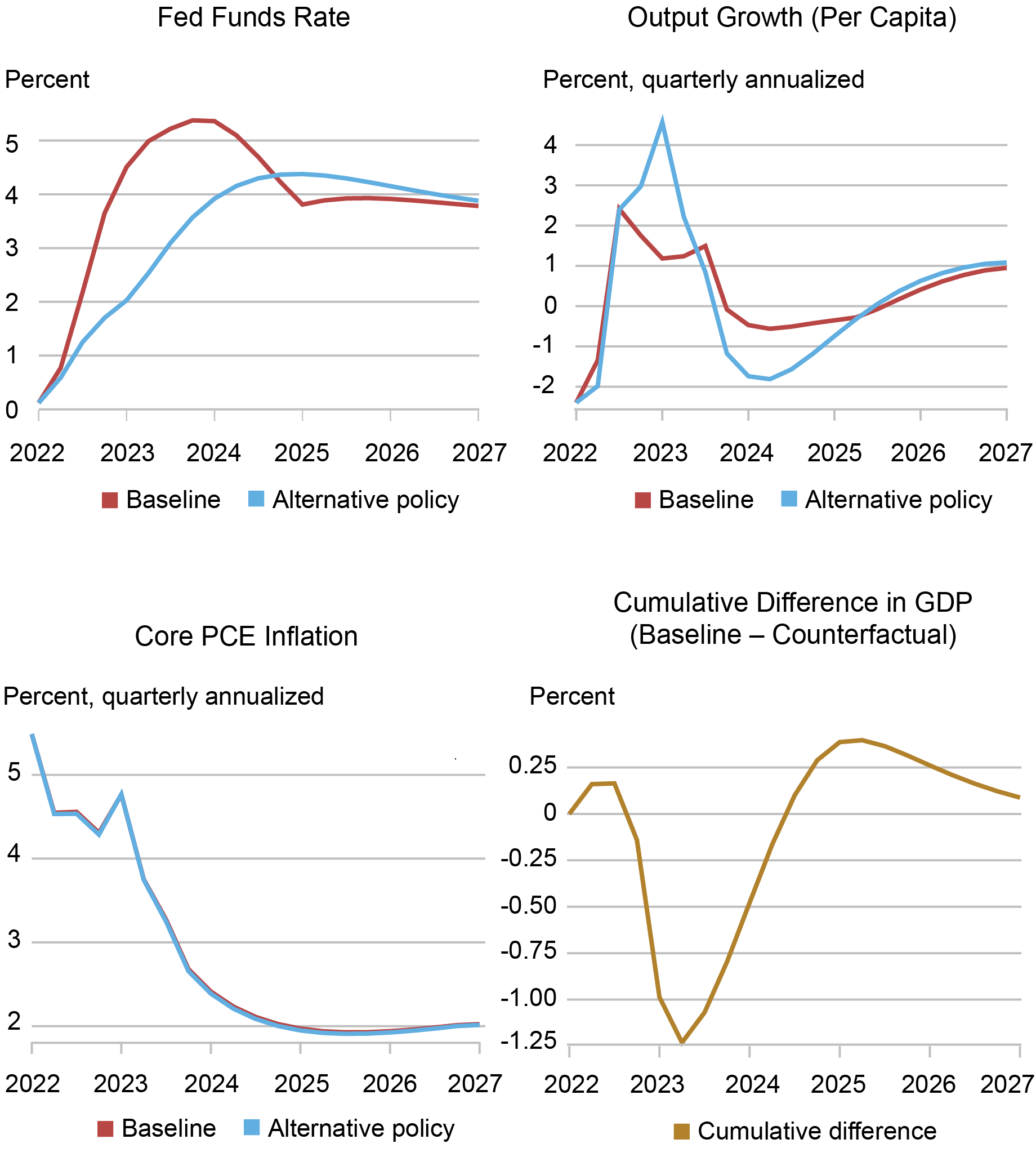
The chart below abstracts from the 2021 ZLB policy and isolates the effect of the aggressive tightening in 2022 and 2023. That is, the DSGE model simulation now starts in 2022:Q2. The chart shows that the pace of tightening in 2022 and early 2023 was more aggressive than implied by the AIT reaction function, even considering the large positive average inflation miss accumulated in the previous quarters. The model allows for both contemporaneous as well as anticipated policy shocks. The former are deviations from the AIT reaction function that take place in the quarter in which they are announced. The latter are shocks to expected future rates–in other words, forward guidance shocks. In the estimation, these anticipated shocks are identified using FFR expectations obtained in each quarter from the most recent Survey of Primary Dealers. According to the model, there were two large contractionary shocks of about 100 basis points, both contemporaneous, in 2022:Q4 and 2023:Q1. Forward guidance shocks did not play a major role in the hiking period, except for a 50-basis point expansionary six-quarter-ahead anticipated shock in 2023:Q2, which explains why the baseline FFR path falls below the AIT-implied path after mid-2024. The fact that most deviations from the reaction function are due to contemporaneous shocks implies that the aggressive hiking cycle had not been anticipated by the public, possibly limiting its effects on the economy.
Counterfactual with AIT Reaction Function Starting in 2022:Q2
Source: Authors’ calculations.
The effect of these policy shocks on economic activity has been restrictive, with their cumulative effect peaking in mid-2023 with the actual level of output being about 1.25 percent below the AIT counterfactual. The gap then narrows sharply from late 2023 and through 2024 as the AIT policy pushes rates higher over this period while the expected baseline path has the policy rate falling. Note that the projected slowdown in growth in late 2023 and 2024 that takes place under the baseline projection is not due to the lagged effects of the rate hikes in 2022 and 2023. Without these rate hikes the slowdown would be even more pronounced, simply because their peak effect on the level of activity has already been reached and so their contribution to growth is actually positive, at least according to the model.
To conclude, in this post we asked what would have happened had the Fed followed an AIT reaction function starting in 2021:Q2. We show that relative to this counterfactual, actual policy was accommodative in 2021 and then contractionary in 2022 and thereafter, and that the combined effect on economic activity of these deviations from the AIT reaction function has been expansionary and remains so according to the model.

Richard K. Crump is a financial research advisor in Macrofinance Studies in the Federal Reserve Bank of New York’s Research and Statistics Group.

Marco Del Negro is an economic research advisor in Macroeconomic and Monetary Studies in the Federal Reserve Bank of New York’s Research and Statistics Group.

Keshav Dogra is a senior economist and economic research advisor in Macroeconomic and Monetary Studies in the Federal Reserve Bank of New York’s Research and Statistics Group.

Pranay Gundam is a research analyst in the Federal Reserve Bank of New York’s Research and Statistics Group.

Donggyu Lee is a research economist in Macroeconomic and Monetary Studies in the Federal Reserve Bank of New York’s Research and Statistics Group.

Ramya Nallamotu is a research analyst in the Federal Reserve Bank of New York’s Research and Statistics Group.

Brian Pacula is a research analyst in the Federal Reserve Bank of New York’s Research and Statistics Group.
How to cite this post:
Richard Crump, Marco Del Negro, Keshav Dogra, Pranay Gundam, Donggyu Lee, Ramya Nallamotu, and Brian Pacula, “The New York Fed DSGE Model Perspective on the Lagged Effect of Monetary Policy,” Federal Reserve Bank of New York Liberty Street Economics, November 21, 2023, https://libertystreeteconomics.newyorkfed.org/2023/11/the-new-york-fed-d....

Why Do Forecasters Disagree about Their Monetary Policy Expectations?

Consumers’ Perspectives on the Recent Movements in Inflation

The New York Fed DSGE Model Forecast— September 2023
Disclaimer
The views expressed in this post are those of the author(s) and do not necessarily reflect the position of the Federal Reserve Bank of New York or the Federal Reserve System. Any errors or omissions are the responsibility of the author(s).
A Bayesian VAR Model Perspective on the Lagged Effect of Monetary Policy

Over the last few years, the U.S. economy has experienced unusually high inflation and an unprecedented pace of monetary policy tightening. While inflation has fallen recently, it remains above target, and the economy continues to expand at a robust pace. Does the resilience of the U.S. economy imply that monetary policy has been ineffectual? Or does it reflect that policy acts with “long and variable lags” and so we haven’t yet observed the full effect of the monetary tightening that has already taken place? Using a Bayesian vector autoregressive (BVAR) model, we show that economic activity has, indeed, been substantially stronger than would have been anticipated considering the rapid policy tightening. Still, the model expects a significant slowdown in 2024-25, even though short-term interest rates are forecasted to fall.
High Inflation and High Growth?
To study the behavior of the U.S. economy over the last few years, we use a large BVAR model that features thirty-five macroeconomic and financial time series, five lags of past data, and is estimated over the sample ranging from the second quarter of 1973 through the end of 2019. For further details see this paper. To answer our question of interest we will rely on so-called “conditional forecasts.” In loose terms, a conditional forecast is the best guess of a future value of a variable when one has knowledge about the future value or values of some other set of variables.
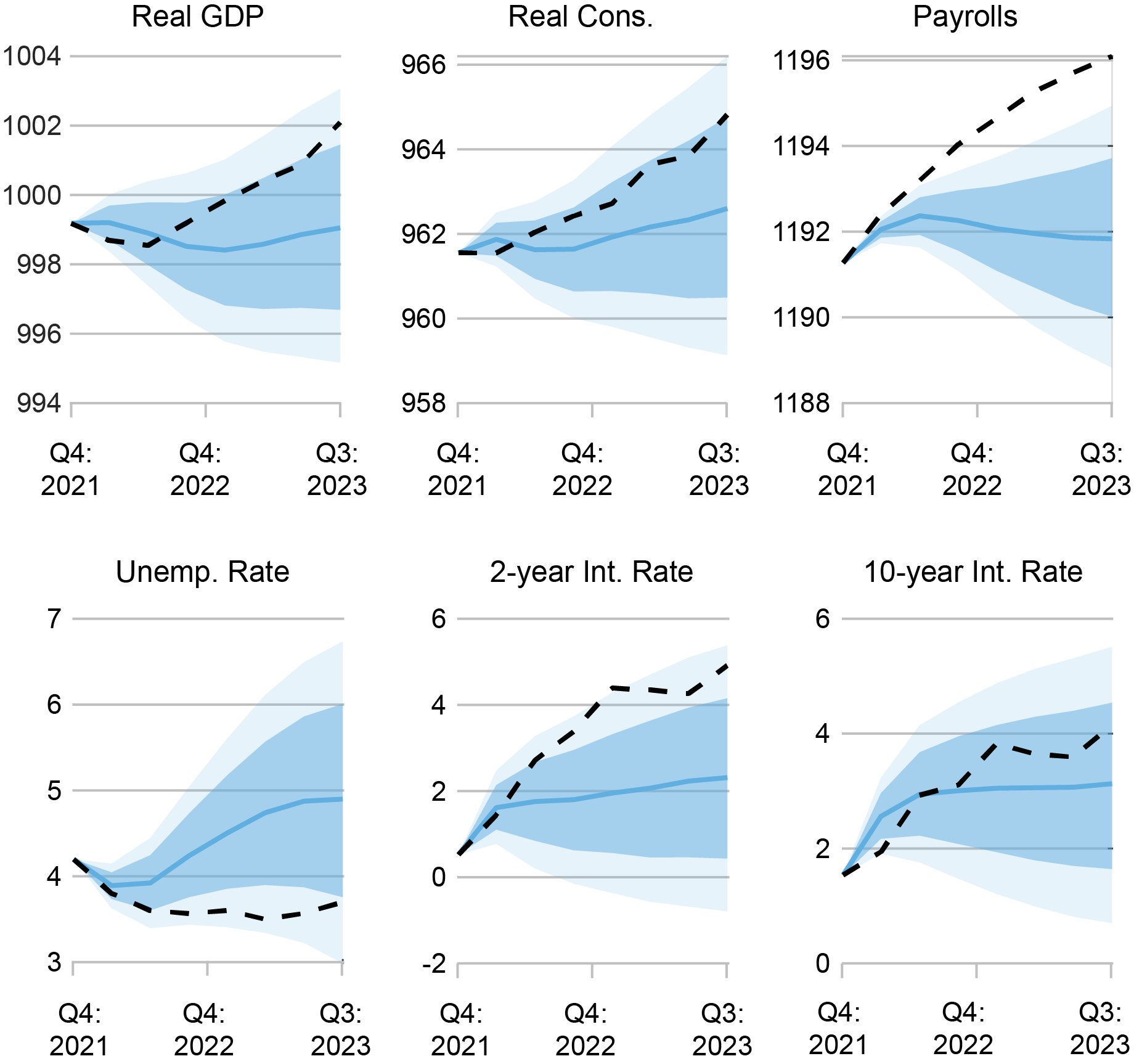
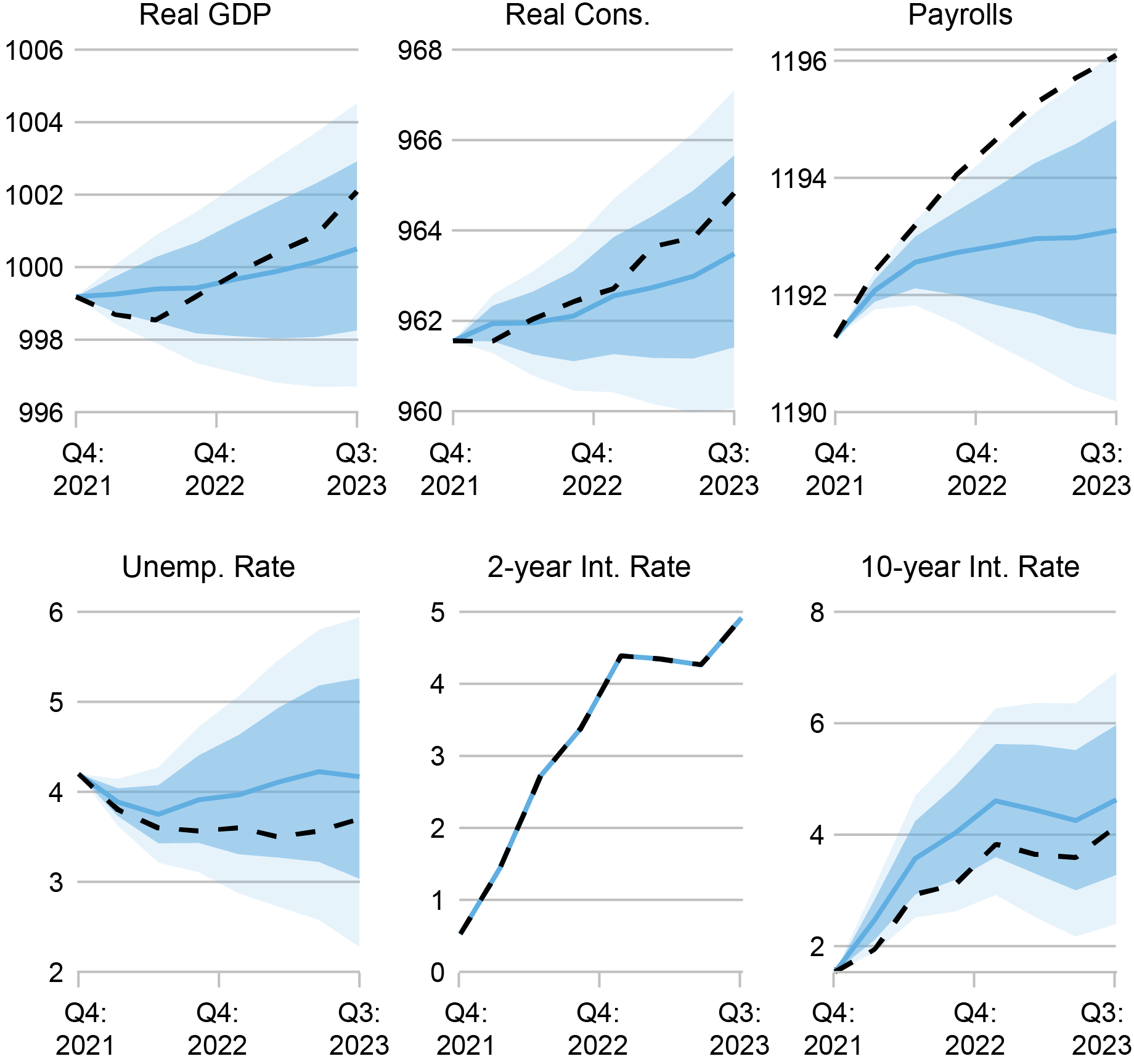
In our first exercise, we feed the model all the historical information available up to the fourth quarter of 2021 and the path of price inflation in 2022 and the first three quarters of 2023. We are asking the model: if you only knew the path of inflation since 2021, what would you predict for other economic and financial series such as real GDP growth, the unemployment rate, or interest rates over these seven quarters? The chart below shows the conditional forecast (blue line) and shaded regions denoting the associated pointwise posterior coverage intervals (dark shading 68 percent and light shading 90 percent). The dashed lines represent the path of the realized data.
2021:Q4 Forecasts Conditional on the Path of Inflation
Sources: Bureau of Economic Analysis; Bureau of Labor Statistics; Board of Governors of the Federal Reserve System; authors’ calculations.
Notes: The chart shows the conditional forecast (blue line) and shaded regions denoting the associated pointwise posterior coverage intervals (dark shading 68 percent and light shading 90 percent). Dashed lines represent the path of the realized data. The top row reports results for the logarithm of real gross domestic product (Real GDP), real personal consumption expenditures (Real Cons.), and nonfarm payrolls (Payrolls). The bottom row reports results for the civilian unemployment rate (Unemp. Rate), the two-year nominal interest rate (2-Year Int. Rate), and the ten-year nominal interest rate (10-Year Int. Rate).
The chart indicates that the model would have anticipated a modest increase in short-term interest rates and a recession, with the level of real GDP falling and the unemployment rate rising to about 5 percent. Intuitively, this reflects the fact that the unusually high inflation observed since 2021 would typically trigger tighter monetary policy, which would in turn lead to a recession. However, the rise in the two-year yield predicted by the model is substantially lower than the realized path: the rise in interest rates that did occur was over and above what would have been foreseen just based on the path of inflation.
High Inflation and Interest Rates and High Growth?
As we saw in the previous chart, short-term interest rates rose to much higher levels than the model would have anticipated based solely on the path of inflation since 2021. As a second exercise, we ask the model what the conditional forecast would be if, in addition to inflation since 2021, we also feed the model the future path of two-year nominal interest rates. This informs the model on the rapid rise in short-term interest rates since late 2021. The chart below presents the results from this exercise. Since we use the future path of the two-year interest rate in forming the forecast, the dashed and solid lines are the same.
2021:Q4 Forecasts Conditional on the Path of Inflation and Two-Year Yields
Sources: Bureau of Economic Analysis; Bureau of Labor Statistics; Board of Governors of the Federal Reserve System; authors’ calculations.
Notes: The chart shows the conditional forecast (blue line) and shaded regions denoting the associated pointwise posterior coverage intervals (dark shading 68 percent and light shading 90 percent). The dashed lines represent the path of the realized data. The top row reports results for the logarithm of real gross domestic product (Real GDP), real personal consumption expenditures (Real Cons.), and nonfarm payrolls (Payrolls). The bottom row reports results for the civilian unemployment rate (Unemp. Rate), the 2-year nominal interest rate (2-Year Int. Rate), and the 10-year nominal interest rate (10-Year Int. Rate).
In contrast to the previous exercise, when conditioning on the higher path of interest rates as well as inflation, the model forecasts only anemic growth but not an outright decline in activity. One interpretation is that the higher path of interest rates—relative to the forecasted path, conditioning on inflation—reflects, in part, a systematic monetary policy response to higher economic activity. Nonetheless, the model is still surprised on the upside by the realized activity data. As shown in the chart, consumption and labor market activity are meaningfully stronger than would be expected. In the center panel in the top row, we observe that realized real consumption has skirted the 68 percent coverage interval, whereas in the bottom left and top right panels the unemployment rate has done the same and payrolls have comfortably exceeded the intervals.
These results indicate that, conditional on the steep increase in short rates and elevated inflation over the past two years, we would have expected to see persistently slower real activity by now, even considering the lags with which monetary policy has acted in the past. This is consistent with the notion that the economy experienced positive demand shocks over this period, which offset the usual effect of tighter policy.
Current Forecast
Do these results imply that without a significant further tightening of policy, we would expect activity and inflation to remain elevated? In the chart below, we report the current forecast based on the data available up to the third quarter of 2023. The forecast features a decline of more than 100 basis points in the two-year interest rate over the next two years. Nonetheless, the forecast features a slowdown in activity and inflation consistent with behavior observed in past slowdowns and NBER-defined U.S. recessions. Specifically, we observe a persistent decline in the level of real GDP (top left panel) starting in early 2024 in conjunction with a rising unemployment rate and a fall in payroll employment (bottom left and top right panels). Looking at the underlying detail (not shown in the chart), the decline in economic activity is led by real investment. Finally, in the chart below we also show the forecasted path for core PCE inflation (bottom right panel). Concomitant with the projected slowdown in real activity, the forecasted path of inflation continues its pre-existing decline and, in fact, falls below the target rate of 2 percent in 2024 and 2025.
Current BVAR Forecast
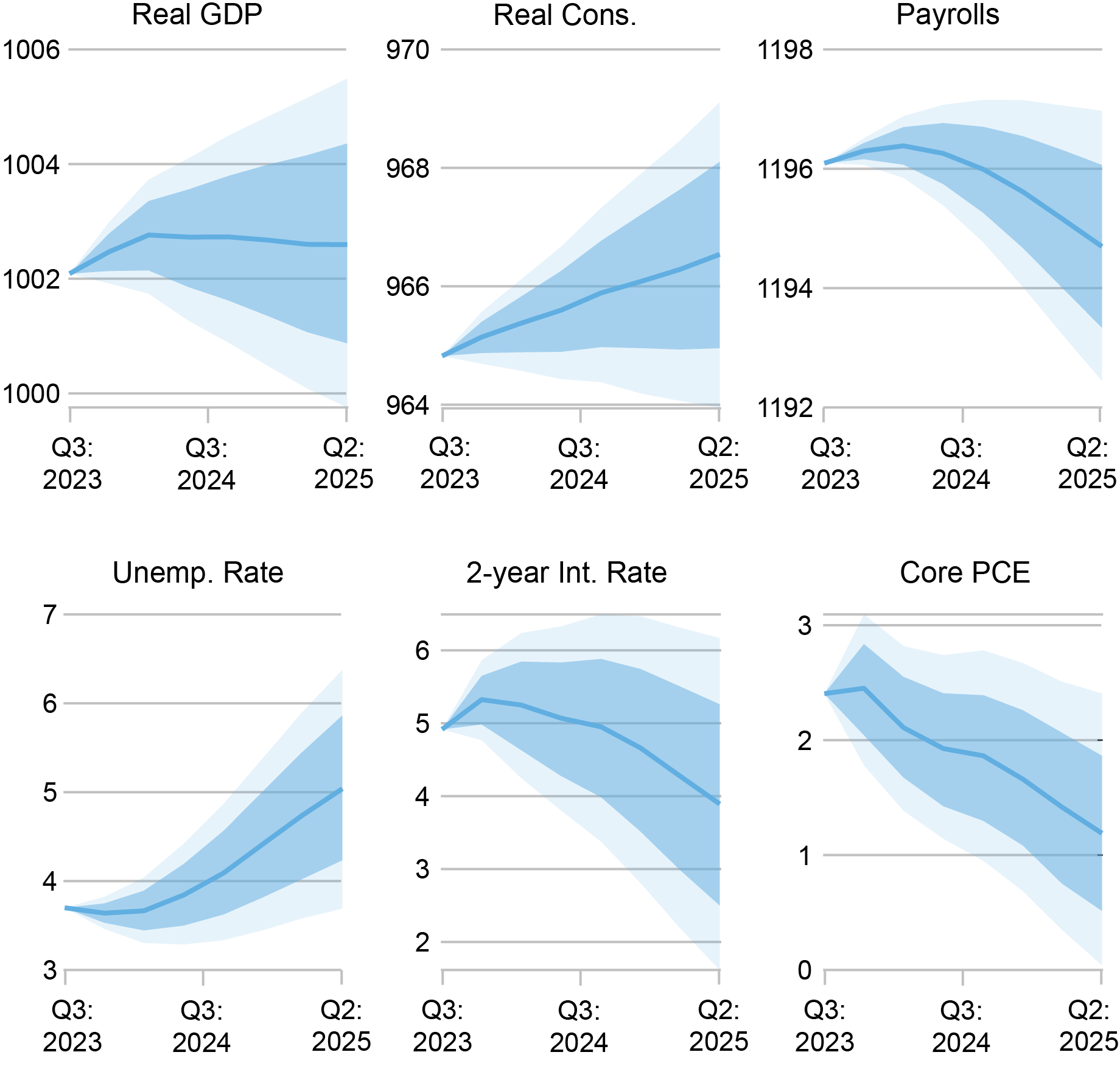
Sources: Bureau of Economic Analysis; Bureau of Labor Statistics; Board of Governors of the Federal Reserve System; authors’ calculations.
Notes: The chart shows the forecast (blue line) and shaded regions denoting the associated pointwise posterior coverage intervals (dark shading 68 percent and light shading 90 percent). The top row reports results for the logarithm of real gross domestic product (Real GDP), real personal consumption expenditures (Real Cons.), and nonfarm payrolls (Payrolls). The bottom row reports results for the civilian unemployment rate (Unemp. Rate), the 2-year nominal interest rate (2-Year Int. Rate), and core PCE inflation (Core PCE).
Conclusion
Taken together, the results from the three forecasting exercises suggest that economic activity in 2022-23 was stronger than expected conditional on the path of interest rates and inflation. But this does not imply that more tightening is required to slow real activity and reduce inflation. While the lagged effects of monetary tightening were counteracted by positive demand shocks in 2023-24, the model still expects a slowdown in 2024-25.
One limitation of our analysis is that the BVAR is a reduced-form model, which means that we cannot conduct a true counterfactual analysis. Said differently, we can’t answer questions such as: what would have happened if monetary policy—and only monetary policy—had been different since 2021? In our accompanying post, we will take an alternative approach that enables us to investigate these types of questions further.
Richard K. Crump is a financial research advisor in Macrofinance Studies in the Federal Reserve Bank of New York’s Research and Statistics Group.
Marco Del Negro is an economic research advisor in Macroeconomic and Monetary Studies in the Federal Reserve Bank of New York’s Research and Statistics Group.
Keshav Dogra is a senior economist and economic research advisor in Macroeconomic and Monetary Studies in the Federal Reserve Bank of New York’s Research and Statistics Group.
Pranay Gundam is a research analyst in the Federal Reserve Bank of New York’s Research and Statistics Group.
Donggyu Lee is a research economist in Macroeconomic and Monetary Studies in the Federal Reserve Bank of New York’s Research and Statistics Group.
Ramya Nallamotu is a research analyst in the Federal Reserve Bank of New York’s Research and Statistics Group.
Brian Pacula is a research analyst in the Federal Reserve Bank of New York’s Research and Statistics Group.
How to cite this post:
Richard Crump, Marco Del Negro, Keshav Dogra, Pranay Gundam, Donggyu Lee, Ramya Nallamotu, and Brian Pacula, “A Bayesian VAR Model Perspective on the Lagged Effect of Monetary Policy,” Federal Reserve Bank of New York Liberty Street Economics, November 21, 2023, https://libertystreeteconomics.newyorkfed.org/2023/11/a-bayesian-var-mod....
A Large Bayesian VAR of the United States Economy
Disclaimer
The views expressed in this post are those of the author(s) and do not necessarily reflect the position of the Federal Reserve Bank of New York or the Federal Reserve System. Any errors or omissions are the responsibility of the author(s).